Counting highlighted cells can be useful when you’re working with color-coded data in Google Sheets. If you’re using colors to mark task status or track progress, it can be difficult to keep an accurate count just by looking at the sheet. Instead of manually going through each cell, you can use a few simple methods to count the colored cells automatically.
In this article, we’ll show you how to count highlighted cells in Google Sheets using practical techniques that help organize your data and make analysis easier.
You can use the built-in COUNTIF function to count highlighted cells based on text values.
Here’s is an easy guide how to apply this method:
➤ Open your dataset in the Google sheets.
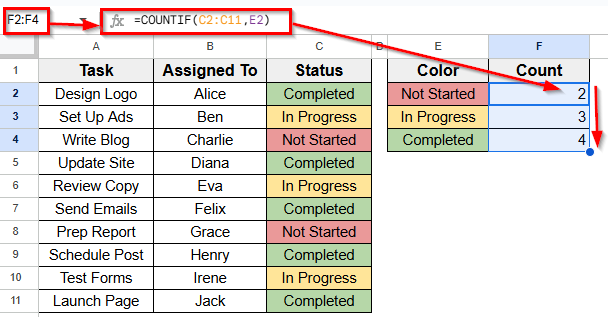
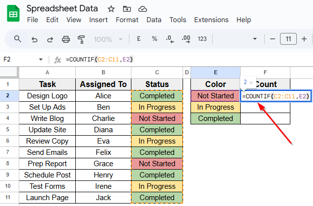
➤ Select an empty cell where you display the result of counting highlighted cells. For example, select cell F2 next to the label Not Started.
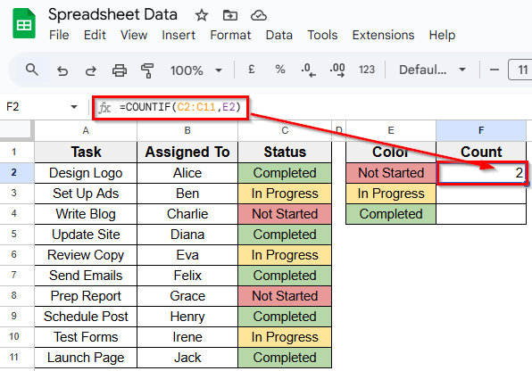
➤ Enter this formula =COUNTIF(C2:C11, E2)
➤ Click Enter. This will return the number of tasks marked as Not Started.
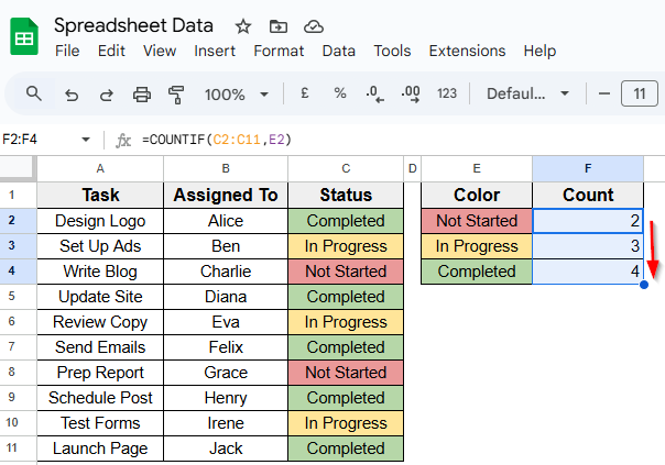
➤ To apply the same formula to the other rows, drag the fill handle from F2 down to F4 and the values will update automatically.
Using Apps Script to Count by Fill Color
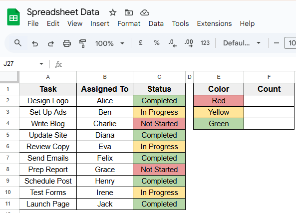
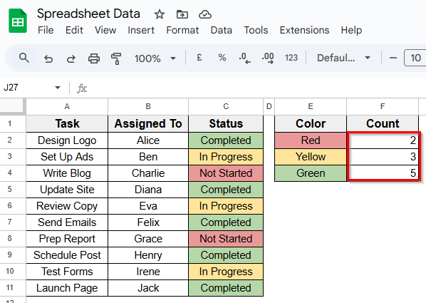
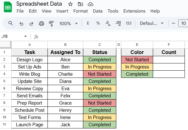
In the following dataset, there is a single sheet with three main columns labeled Task, Assigned To, and Status. Each row represents a task assigned to a team member, with the Status column filled using color to indicate progress. Green is used for completed tasks, yellow for tasks in progress, and red for those not started.
To make it easier to count the colored cells, a small color key is included on the right side of the sheet. This section contains the three colors used in the Status column, along with an empty cell next to each one where the final count will be displayed.
We’ll use this setup to apply and practice different methods for counting highlighted cells in Google Sheets.
You can use Apps Script method to count how many times a specific background color appears in your dataset. The script will check the Status column, compare each cell’s background color to a reference color, and return the total count.
Here’s a simple step-by-step guide to apply this method:
➤ Open your dataset in Google sheets.
➤ Go to the top Menu and click Extensions >> Apps Script.
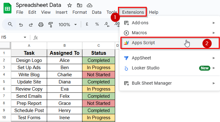
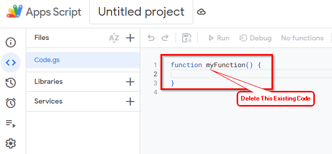
➤ The Apps Script editor will open in a new tab. Delete any code already in the editor.
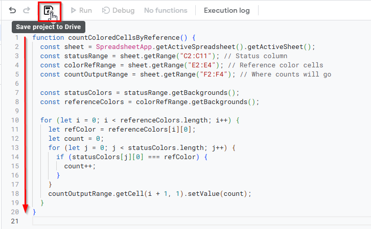
➤ Copy and paste the script below into the editor:
function countColoredCellsByReference() {
const sheet = SpreadsheetApp.getActiveSpreadsheet().getActiveSheet();
const statusRange = sheet.getRange("C2:C11"); // Status column
const colorRefRange = sheet.getRange("E2:E4"); // Reference color cells
const countOutputRange = sheet.getRange("F2:F4"); // Where counts will go
const statusColors = statusRange.getBackgrounds();
const referenceColors = colorRefRange.getBackgrounds();
for (let i = 0; i < referenceColors.length; i++) {
let refColor = referenceColors[i][0];
let count = 0;
for (let j = 0; j < statusColors.length; j++) {
if (statusColors[j][0] === refColor) {
count++;
}
}
countOutputRange.getCell(i + 1, 1).setValue(count);
}
}
➤ Click the Save icon.
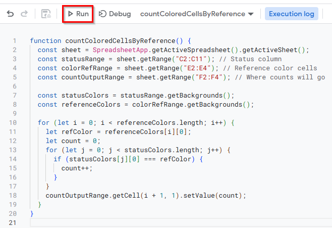
➤ Once you save the script the Run option will activate.
➤ Click Run to execute the script.
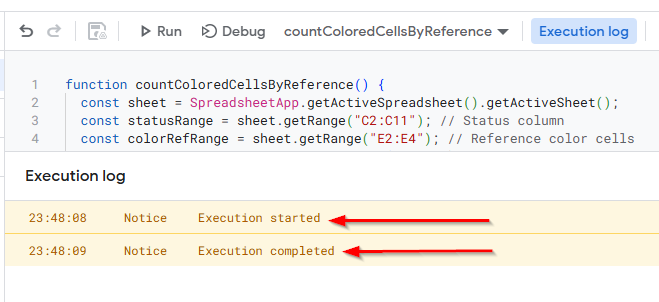
➤ Now, you’ll see a message saying Execution started at the top of the editor.
Note:
If this is your first time running the script, a prompt will appear asking you to review and grant permission. Click Continue to allow the execution.
➤ Now, go back to your spreadsheet, and you’ll see the total count of each color displayed in column F, next to the matching color key in column E.
Using the Function by Color Add-On
The Function by Color add-on is a simple way to count colored cells in Google Sheets. It lets you count or sum cells based on their background color.
Here’s how to use this tool in 2 steps:
Step 1: Install the Function by Color
➤ Open your Google sheets file where you have a dataset with highlighted cells.
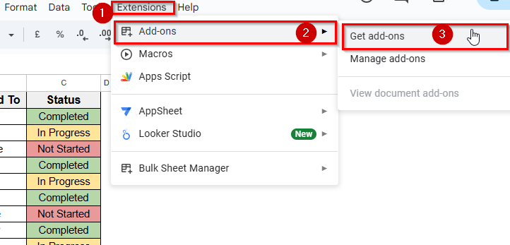
➤ Go to the top Menu, and click Extensions >> Add-ons >> Get add-ons.
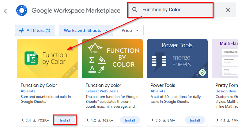
➤ Search for Function by Color in the Google Workspace Marketplace.
➤ Click Install and approve the required permissions.
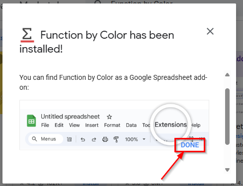
➤ Once installed, the add-on will be listed under your Extensions menu.
➤ Click Done.
Step 2: Use Function by Color Tool to Count Highlighted Cells
➤ Go back to your Spreadsheet.
➤ Next, go to the top Menu, and click Extensions >> Function by Color >> Start.
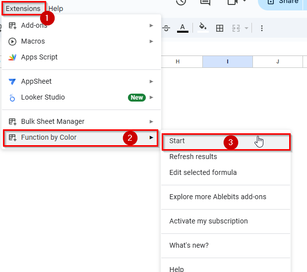
➤ A sidebar will appear on the right side of your screen.
➤ In the Select range box, enter your colored cell range. For example, type C2:C11. ➤ In the Select color box, use the color picker to select the specific color you want to count.
➤ From the Use Function dropdown menu, choose COUNTA (text).
➤ In the Paste result to field, enter the cell where you want to display the result. For example, type F2.
➤ Next, click the Insert Function button at the bottom of the sidebar.
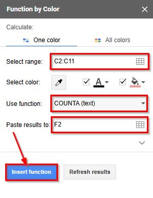
➤ You’ll now see the total number of cells with the selected background color appear in that cell.
Note:
Repeat the process for each color in your reference list by updating the range, choosing a new color, and selecting a new result cell.
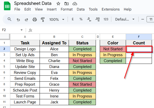
Using COUNTIF Function to Count Highlighted Cells by Text Value
In this version of the dataset, only the Color column has been updated to display text labels such as Not Started, In Progress, and Completed. It now shows the matching status values found in the main table. These labels represent each category of task status.
We’ll use this setup to apply the method for counting highlighted cells based on text values using a simple built-in formula in Google Sheets.
COUNTIF function is a simple built-in method to count highlighted cells in Google sheets based on text. If the colored cells in your dataset also contain consistent text values like Completed, In Progress, or Not Started, you can use the built-in COUNTIF function to count them. This method focuses on the text content inside the cells rather than their background color.
Here’s is an easy guide how to apply this method:
➤ Open your dataset in the Google sheets.
➤ Select an empty cell where you display the result of counting highlighted cells. For example, select cell F2 next to the label Not Started.
➤ Enter this formula =COUNTIF(Range, Cell_Text). For example, type the following formula
=COUNTIF(C2:C11, E2)
➤ Click Enter. This will return the number of tasks marked as Not Started.
➤ To apply the same formula to the other rows, drag the fill handle from F2 down to F4 and the values will update automatically.
Frequently Asked Questions
How do I count the number of highlighted cells in Google Sheets?
You can count highlighted cells in Google Sheets using a custom Apps Script. Here’s a simple steps to apply this method:
➤ Open your Google Sheet and go to the top Menu.
➤ Click on Extensions >> Apps Script.
➤ Delete any existing code and paste your script.
➤ Click the Save icon to save the script.
➤ Next, click the Run button to execute the script.
➤ Now, go back to your spreadsheet and you’ll see the result.
How to select only highlighted cells in Google Sheets?
There’s no direct way to select only highlighted cells, but here’s a simple workaround:
➤ Apply a filter to your dataset by clicking Data >> Create a filter.
➤ Click the filter icon on your column header.
➤ Choose Filter by color > Fill color, and select the highlighted color.
This will display only the rows with the highlighted cells, which you can copy or work with as needed.
Wrapping Up
These simple methods help you count highlighted or color-coded cells in Google Sheets. If you’re tracking colors visually, the Function by Color add-on makes it easy without any formulas.
And when you need more flexibility, a custom Apps Script lets you count by filling color directly. The COUNTIF function works best when your sheet uses consistent text values, as it counts based on the cell content rather than background color.
Each method offers a different level of control, depending on how your data is structured. By learning how to apply these techniques, you can keep your spreadsheets more easier to work with.