In Google Sheets, you can return a specific value in one column based on the background color of a cell in another column, such as flagging a row if a cell is red. While this seems simple, it’s not something standard formulas like IF or COUNTIF can handle. This is because visual formatting (like background color) is not accessible via formulas.
In this article, we’ll walk through different methods to detect if a cell is red and return a corresponding value, ranging from custom Apps Script to third-party add-ons. These techniques are perfect for workflows where colors represent status, urgency, or errors, and you need to automate responses based on visual cues in your sheet.
Steps to check for red-colored cells in Google Sheets using the markRedStatuses() Apps Script:
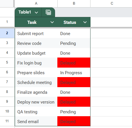
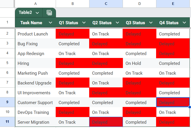
➤ Start with a dataset in cells A1:B11, where column B contains status values like “Delayed,” some of which are colored red.
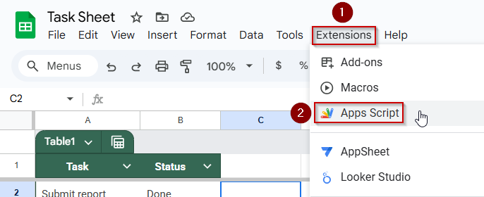
➤ Open the script editor by navigating to Extensions >> Apps Script.
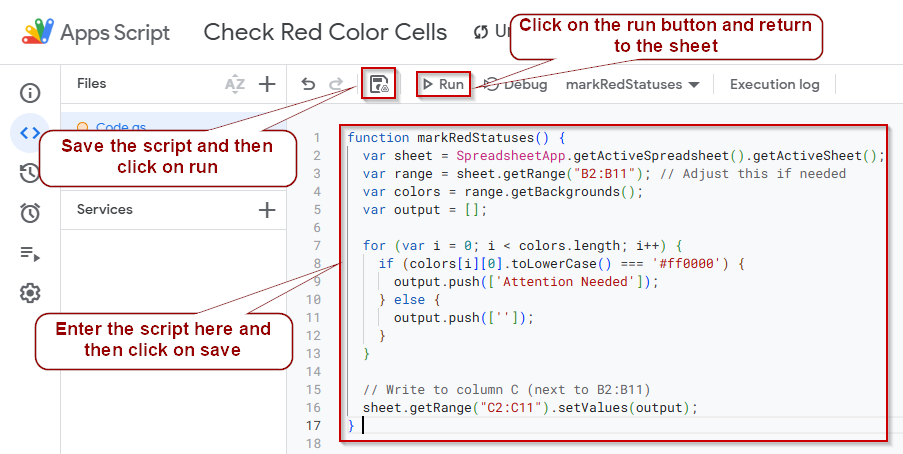
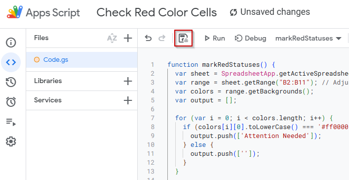
➤ Paste the following script in the editor:
function markRedStatuses() {
var sheet = SpreadsheetApp.getActiveSpreadsheet().getActiveSheet();
var range = sheet.getRange("B2:B11"); // Adjust this if needed
var colors = range.getBackgrounds();
var output = [];
for (var i = 0; i < colors.length; i++) {
if (colors[i][0].toLowerCase() === '#ff0000') {
output.push(['Attention Needed']);
} else {
output.push(['']);
}
}
sheet.getRange("C2:C11").setValues(output);
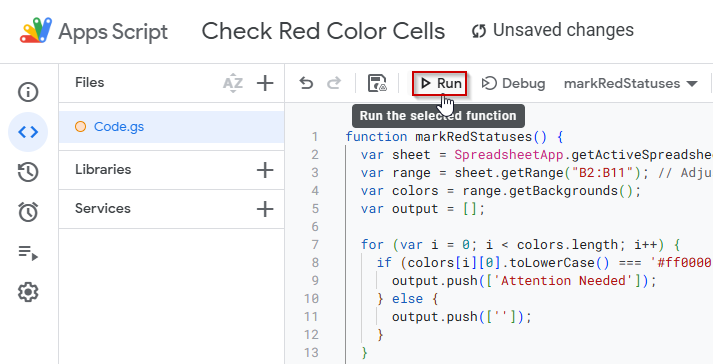
}➤ Save the script, then run it from the toolbar to execute it.
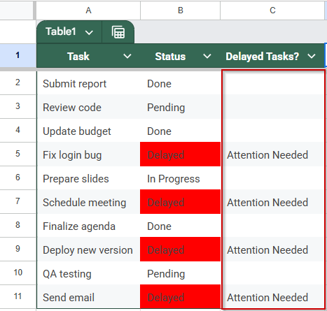
➤ The script checks if each cell in B2:B11 has a red background. If it does, it writes “Attention Needed” in the corresponding row of column C.
Use Apps Script to Check If Cell Color is Red and Return a Value
When you want to perform an action based on cell color in Google Sheets, formulas alone won’t work because they can’t read cell formatting like color. Instead, you can use Google Apps Script to create a custom function that checks if a cell’s background color is red and returns a specific value, such as “Attention Needed,” in another column. This method is dynamic and updates when you run the script, making it useful for tracking statuses like delayed tasks.
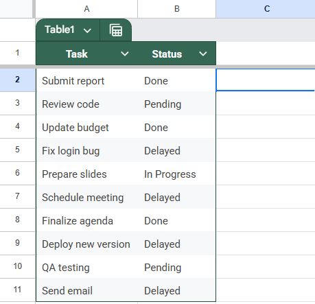
This is the dataset we will be using to demonstrate the methods:
Steps:
➤ Open your Google Sheet with the dataset (Tasks in column A and Status in column B, where “Delayed” cells are colored red).
➤ Go to Extensions >> Apps Script to open the script editor.
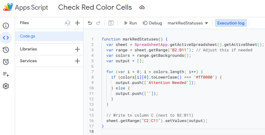
➤ Paste this function in Apps Script:
function markRedStatuses() {
  var sheet = SpreadsheetApp.getActiveSpreadsheet().getActiveSheet();
  var range = sheet.getRange("B2:B11"); // Adjust this if needed
  var colors = range.getBackgrounds();
  var output = [];
  for (var i = 0; i < colors.length; i++) {
    if (colors[i][0].toLowerCase() === '#ff0000') {
      output.push(['Attention Needed']);
    } else {
      output.push(['']);
    }
  }
  // Write to column C (next to B2:B11)
  sheet.getRange("C2:C11").setValues(output);
}
➤ Save the script by clicking on the floppy disk icon, then return to your sheet.
➤ Click on Run.
➤ Go back to the sheet. The script will return “Attention Needed” for all rows where the status cell background is red.
➤ This method is ideal when you want to base conditional outputs on cell color, something not possible with native formulas alone.
Implement Conditional Formatting and Helper Column for Color Detection
Because Google Sheets formulas cannot directly detect cell background colors, you can mimic this by using Conditional Formatting rules to highlight cells with a red color based on their content or conditions. Then, add a helper column that uses a formula to check the same condition and return a specific value. This method leverages the logic behind coloring, rather than reading the color itself, to automate results without scripts.
We have removed the red colours from our dataset for this method as we will add them again through conditional formatting.
Steps:
➤ Select the range where you want to apply the red color formatting (for example, B2:B11).
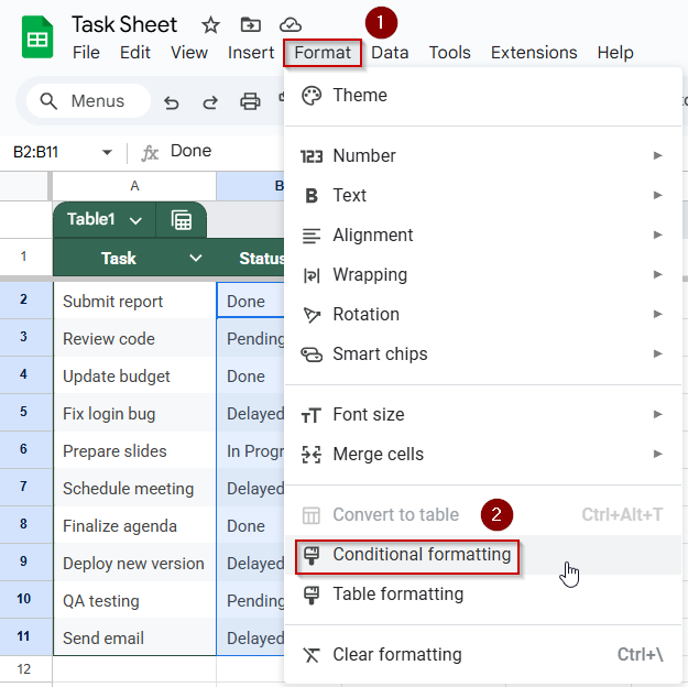
➤ Go to Format >> Conditional formatting.
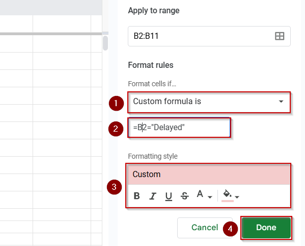
➤ In the Conditional format rules sidebar, under “Format cells if,” select Custom formula is.
➤ Enter the formula that matches your criteria for red cells, for example:
=B2=”Delayed”
➤ Choose a red fill color and click Done. The cells with the value “Delayed” will now be colored red.
➤ In the adjacent helper column (for example, C2), enter this formula to return a specific value when the condition is met:
=IF(B2=”Delayed”, “Check Status”, “”)
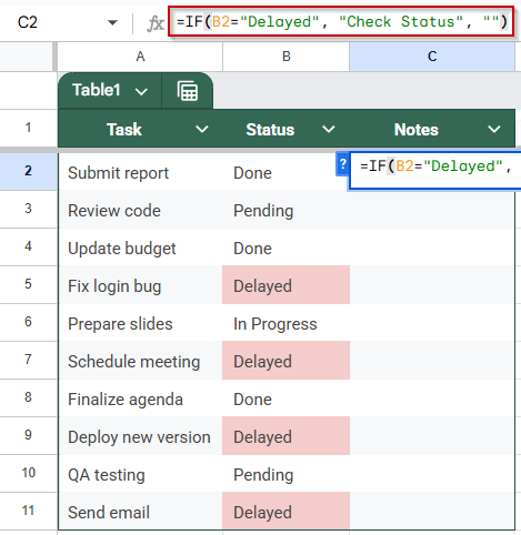
➧ IF(A2="Delayed", "Check Status", "") checks if the cell contains "Delayed" and returns "Check Status" if true, or leaves it blank otherwise.
➧ Adjust the conditional formatting formula and the IF condition to fit your specific criteria and dataset.
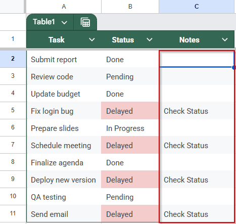
➤ Press Enter and drag the formula down alongside your data range. The helper column will now show “Check Status” next to any cell with “Delayed,” matching your red color formatting.
Use the “Function by Color” Add-on to Return Values Based on Cell Color
If you want to perform calculations or return specific text based on a cell’s background color without using Apps Script, the Function by Color add-on is a great option. It allows you to apply custom functions that recognize cell fill color directly in Google Sheets formulas.
This is the dataset we will be using for this method:
Steps:
➤ Open your Google Sheet.
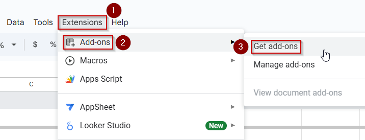
➤ Go to Extensions >> Add-ons >> Get add-ons.
➤ In the Google Workspace Marketplace, search for Function by Color.

➤ Click Install, and follow the prompts to authorize the add-on.
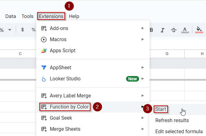
➤ After installation, go to Extensions >> Function by Color >> Start to open the sidebar.
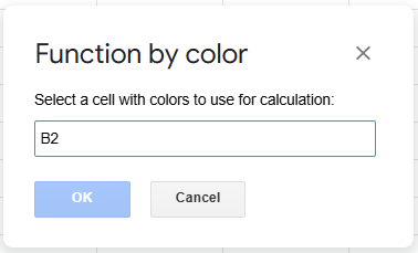
➤ In the sidebar, select the range where red-colored cells are located (e.g., B2:B11).

➤ Click on the color dropper and select the cell that contains the red color.
➤ Select COUNTA (Text) from the ‘Use Function’ field.
➤ Select cells C2:C11 in the ‘Paste results in’ field.
➤ Select each row in the ‘Calculate in’ field.
➤ Uncheck ‘Fill results with your pattern colors’.
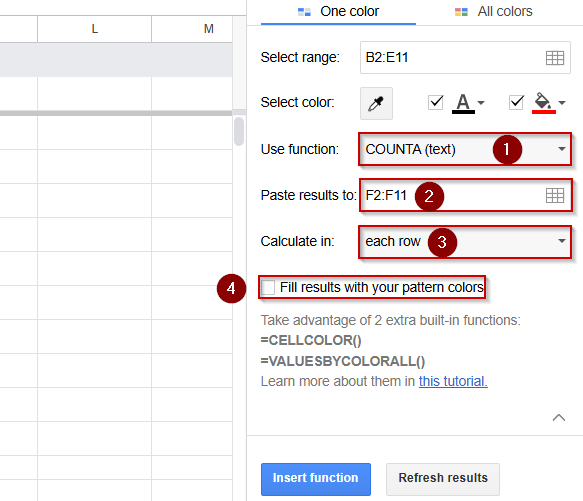
➤ Click on Insert Function.
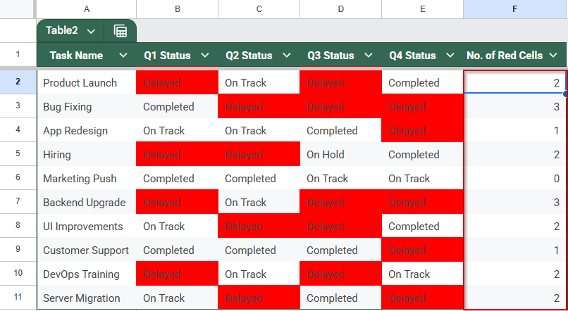
The cells that are red colored will now have the number 1 next to them. This is very useful in a larger dataset.
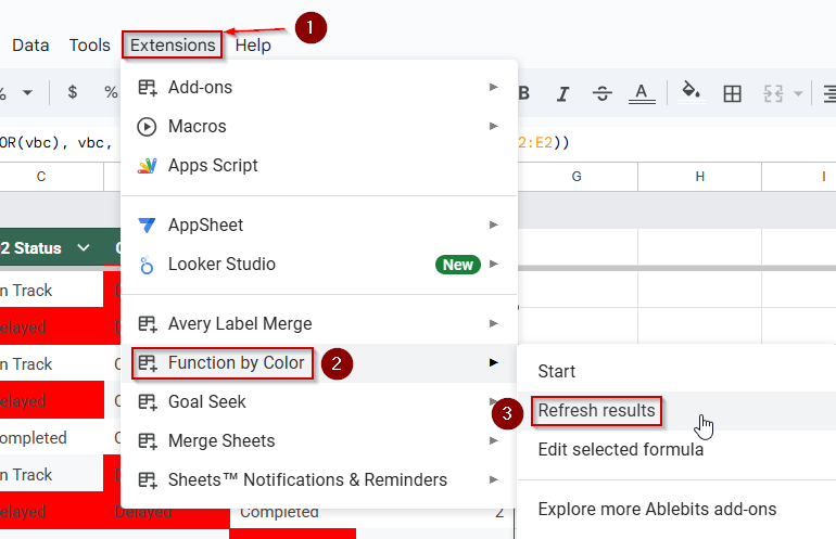
➤ Whenever you change cell colors, go to Extensions >> Function by Color >> Refresh results to update the formula outputs.
Frequently Asked Questions
Can Google Sheets detect cell background color using a formula?
No, Google Sheets formulas cannot detect cell background colors. You need to use Google Apps Script or add-ons for color-based logic and automation.
How do I return a value based on cell color in Google Sheets?
You can’t use formulas for this. Instead, use Apps Script to check the cell color, then return a value in another column based on that condition.
Is there a way to filter by cell color in Google Sheets?
Yes, use the filter feature and select “Filter by color.” However, this works manually and doesn’t support dynamic filtering via formulas.
What’s the best alternative to formulas for color-based conditions?
The best alternative is using a helper column with specific text values and applying conditional formatting for color. This allows formula compatibility and better control.
Wrapping Up
While Google Sheets formulas can’t directly evaluate cell colors, you can still create color-based logic using Apps Script or by redesigning your sheet with helper columns and conditional formatting. Whether you’re flagging delayed tasks or highlighting key values, combining visual cues with script automation or structured data makes your spreadsheets both functional and user-friendly. By understanding the limitations and leveraging the right tools, you can efficiently return specific values based on color and enhance the clarity of your reports or dashboards.