When working in Google Sheets, you’ll often come across duplicate entries. A product name might appear several times in sales data, a customer may place multiple orders, or the same city might be listed repeatedly in a delivery record. These duplicates can make your sheet cluttered and harder to analyze.
Filtering unique values helps you keep the data clean and organized. This allows you to create cleaner reports and quickly summarize key information.
In this guide, we’ll learn different methods to filter unique values in Google Sheets.
Here’s how to filter unique values using the UNIQUE function:
➤ Open your dataset in Google Sheets.
➤ Select the cell F2 or another cell where you want the unique list to appear.
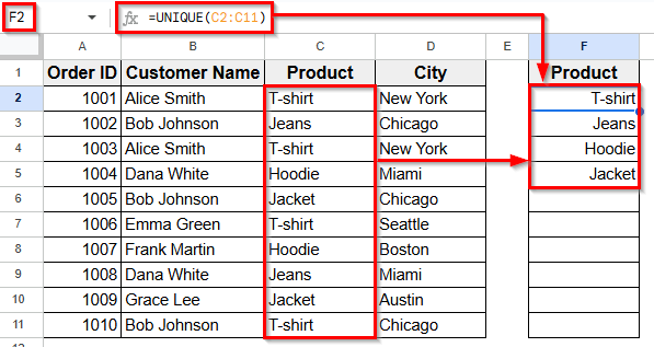
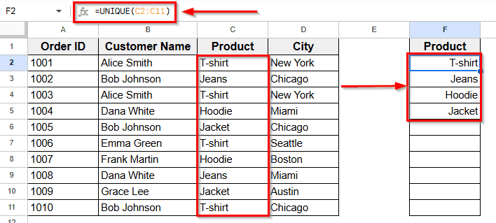
➤ Enter this formula =UNIQUE(C2:C11)
➤ Press Enter.
➤ Google Sheets will instantly return only the unique product names from Column C.
➤ The result will be shown in an array with the outputs- T-shirt, Jeans, Hoodie & Jacket.
Using the UNIQUE Function to Filter Unique Values
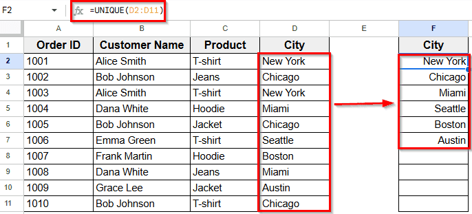
In the following dataset, we have a simple sales record. Column A lists the Order IDs, Column B shows the Customer Names, Column C contains the Products, and Column D shows the Cities.
Column F is currently empty, and we’ll enter different formulas here to filter and display the unique values.
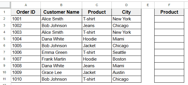
We’ll use this dataset to demonstrate different ways to filter unique values in Google Sheets.
The UNIQUE function is the easiest and most commonly used way to filter distinct values in Google Sheets. It takes a range of data, removes duplicates, and returns only the unique entries in a new column. This method is dynamic, meaning if your dataset changes, the unique list will update automatically.
Here’s how to apply this method:
➤ Open your dataset in Google Sheets.
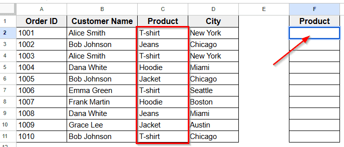
➤ Click on cell F2, where you want the list of unique products from Column C to appear.
➤ Enter the following formula:
=UNIQUE(C2:C11)
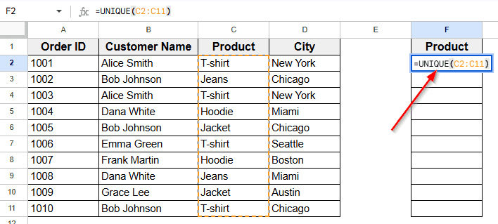
➤ Press Enter. Google Sheets will instantly generate a list of unique products from Column C.
➤ And you’ll get the desired result.
➤ If you add another product in Column C later, the UNIQUE function will automatically update Column F to include it.
Using Filter Tool to Show Unique Values
Another simple way to filter unique values is using Google Sheets Filter UNIQUE function. It allows you to display only the data that meets certain criteria. Unlike formulas, this method doesn’t require writing functions.
Here’s how to apply this method:
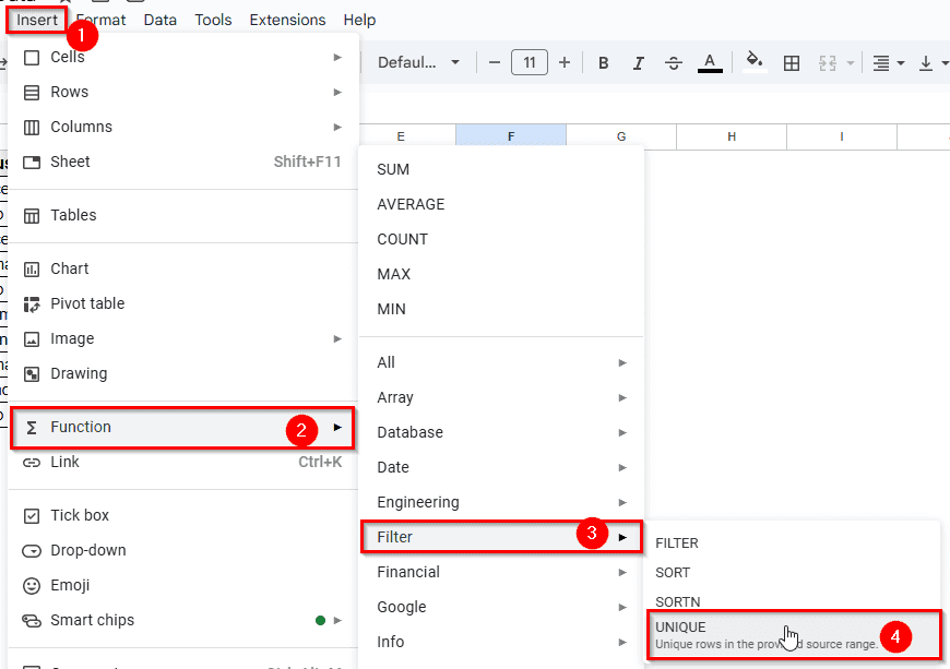
➤ Open your dataset in Google Sheets.
➤ Click on cell F2, where you want the list of unique city names to appear.
➤ Go to the Home tab, and click Insert >> Function >> Filter >> UNIQUE.
➤ Cell F2 displays this formula UNIQUE( ) automatically.
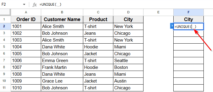
➤ Enter the cell range such as D2:D10 in the bracket. For example, UNIQUE(D2:D11).
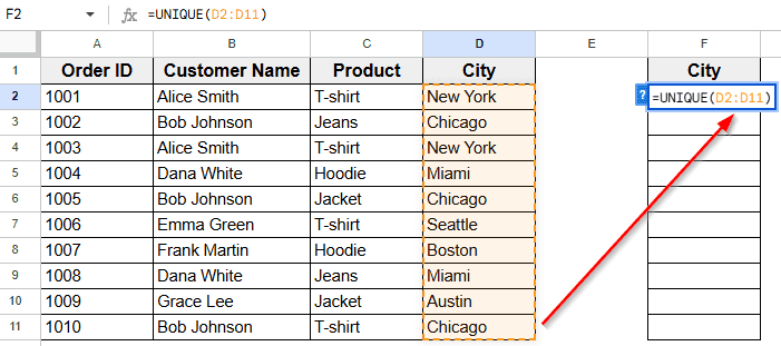
➤ Press Enter. Now, you’ll see the unique city names in Column F.
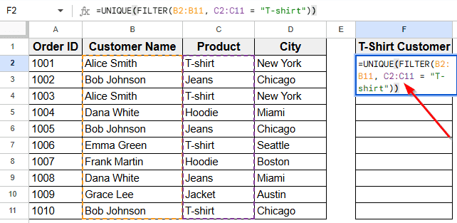
Filter Unique Values Based on a Condition
You can filter unique customer names based on a condition by combining the UNIQUE and FILTER functions. This lets you display only the customers who purchased T-shirts without duplicates.
Here’s how to apply this method:
➤ Open your dataset in Google Sheets.
➤ Click on cell F2, where you want the filtered list of T-shirt Customer names to appear.
➤ Enter the following formula:
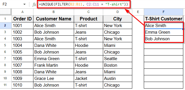
=UNIQUE(FILTER(B2:B11, C2:C11 = "T-shirt"))
➤ Press Enter. Google Sheets will instantly generate a list of unique customer names from Column B who purchased T-shirts in Column C.
➤ If you add another T-shirt purchase later, the formula will automatically update Column F to include it.
Frequently Asked Questions
How can I filter unique customer names who purchased a specific product?
To filter unique customer names for a specific product, use the formula:
=UNIQUE(FILTER(B2:B11, C2:C11=”Product Name”))
For example, to filter customers who bought T-shirts:
=UNIQUE(FILTER(B2:B11, C2:C11=”T-shirt”))
It returns a list of unique customer names who purchased that product.
Can I filter unique customer names for multiple products at once?
Yes, you can use the FILTER function with multiple conditions. For example:
=UNIQUE(FILTER(B2:B11, (C2:C11=”T-shirt”) + (C2:C11=”Jeans”)))
This will return unique names of customers who purchased either T-shirts or Jeans.
Will the list of unique customer names update automatically?
Yes. The formula using UNIQUE and FILTER is dynamic. If you add new purchases or names in the dataset, the filtered list will automatically update.
Wrapping Up
Filtering unique values in Google Sheets is a simple way to clean up your data and make it easier to analyze. Using the UNIQUE function quickly removes duplicates. Also, combining the UNIQUE function with FILTER function allows you to focus on specific conditions, like customers who purchased a certain product.
These methods help keep your datasets organized and save time when working with large amounts of data. Choose the method that suits you best to generate accurate reports, build targeted summaries, or manage customer lists.