When making decisions, it’s important to understand how different factors can impact your results. In Google Sheets, you can use powerful what-if analysis methods like data modeling, Goal Seek, and sensitivity analysis to explore various possibilities. These tools help you test assumptions, find target values, and see how changes in one variable affect others. In this article, we’ll guide you through each method so you can make smarter, data-driven decisions with ease.
What Is What if Analysis in Google Sheets?
What if analysis in Google Sheets is a way to test how changing one or more input values affects the results in your spreadsheet. It helps you explore different scenarios without changing your original data. Suppose you run a bakery and want to know how your profit changes if you raise your prices. Now, if you change the profit margin from 20% to 30%, the selling price updates automatically. This illustrates how a small change in input can impact your revenue, a classic application of what-if analysis.
Types of What-If Analysis in Google Sheets
What if analysis allows you to test different scenarios by adjusting values in your spreadsheet to see how results change. In Google Sheets, two common types of what if analysis are scenario analysis and sensitivity analysis. Both help you make smarter decisions, but they focus on different ways of testing your data.
Scenario Analysis
Scenario analysis involves changing multiple variables at once to model different situations. Suppose you create three cases: Best Case (high sales, low cost), Worst Case (low sales, high cost), and Expected Case (average values), and observe how each scenario affects your profit.
Sensitivity Analysis
Sensitivity Analysis tests how changing just one variable impacts the result, while keeping all other inputs constant. You adjust only the profit margin and watch how it affects the total profit, helping you identify how sensitive your outcome is to that specific input.
Scenario-Based Data Modeling for What-If Analysis in Google Sheets
Data modeling in Google Sheets lets you explore how changes in key inputs affect your results. Instead of sticking to just one version of your data, you can create multiple what-if setups and switch between them easily. In this section, we’ll show you how to model different scenarios using manual input changes, dropdown selections, and a simple scenario manager.
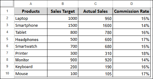
Suppose we have a dataset containing: Products, Sales Target, Actual Sales, and Commission Rate. Now we will explore different scenarios to see how changes in sales or commission rates affect overall earnings and performance.
Manual Input Changes
Manual input changes let you directly edit values in your sheet to see how they affect the results. It is the simplest way to test different scenarios without any setup.
➤ Choose a cell and put the following formula to get the bonus for each product.
=IF(C2>=B2, (C2-B2)*VALUE(D2), 0)
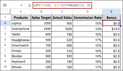
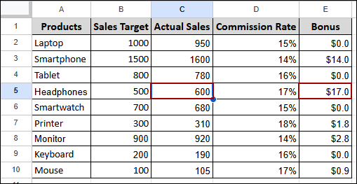
Now, change any actual sales value, and you will see the bonus amount changing according to it. Thus, you can instantly test different outcomes and make informed decisions based on the results.
Dropdown Scenarios
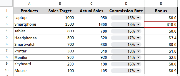
Here, we are creating a dropdown for the commission rate, so you can easily test different percentages. As you select a new rate, the bonus calculations update automatically based on your choice.
➤ Select cells D2:D10 and click Data > Data validation from the menu bar.
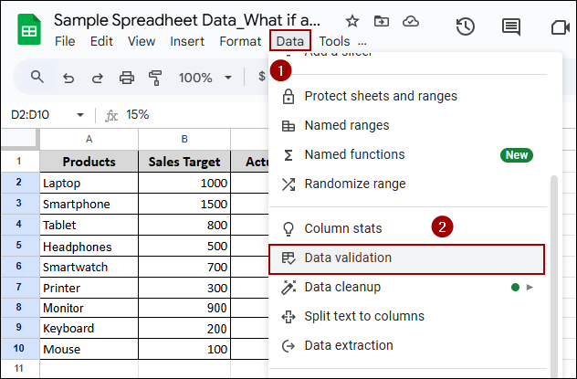
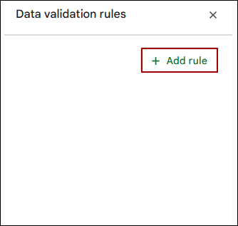
➤ Now, hit the Add rule option.
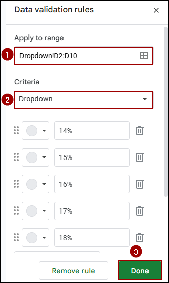
➤ Then, choose Apply to range, Criteria and click Done.
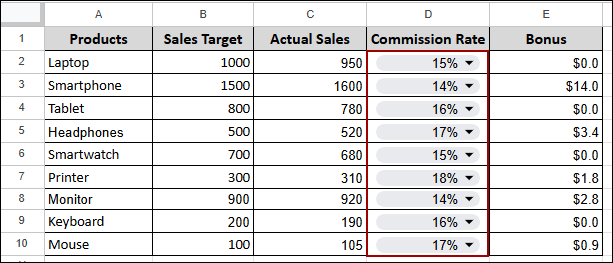
Thus, a drop-down will be created for all the cells in the commission rate column.
➤ To clearly see the changes, choose any drop-down cell and select a different value.
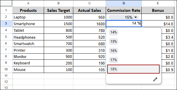
The sheet will instantly update the bonus amount for the row, helping you compare different commission scenarios with ease.
Scenario Manager (Manual Table + Dropdown)
Scenario manager lets you organize multiple scenarios in a table and apply them using a dropdown. It’s a structured way to switch between different sets of inputs without editing the data manually each time.
Suppose we have the same dataset but a blank column for Actual Sales. Below we have three sales scenarios (Best Case, Expected, Worst Case) for each product, providing projected Actual Sales figures under each scenario. Here, we will create a dropdown list to switch between different sales scenarios. Then, we will analyze this dataset to compare actual sales across different sales scenarios for each product.
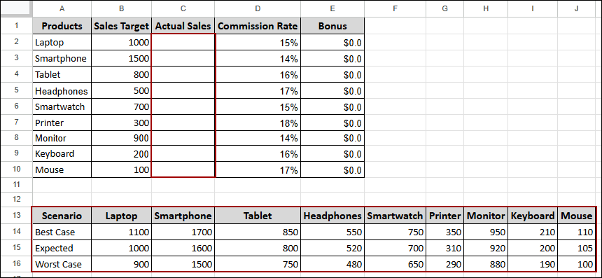
To create a dropdown list in cell G2,
➤ Select cell G2, click Data > Data validation from the menu bar.
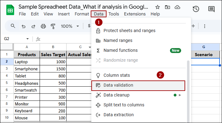
As a result, the Data validation rules sidebar will appear.
➤ In the dropdown options, input your scenarios: Best Case, Expected, and Worst Case. You can also assign colors to each option if desired.
➤ Finally, click Done.
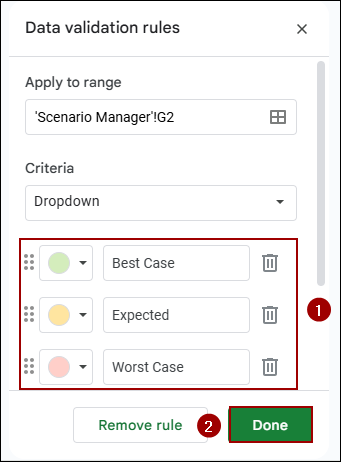
Thus, a dropdown menu containing your defined scenarios will be created in cell G2. Now, we will link the selected scenario from the dropdown to automatically populate the Actual Sales column using a formula.
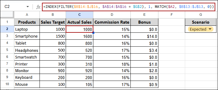
➤ Select cell C2 and enter the following formula into the cell.
➤ Then, drag down to fill.
=INDEX(FILTER($B$14:$J$16, $A$14:$A$16 = $G$2), 1, MATCH($A2, $B$13:$J$13, 0))
The above formula will dynamically fetch the corresponding Actual Sales value from the Scenario table based on the product in column A.
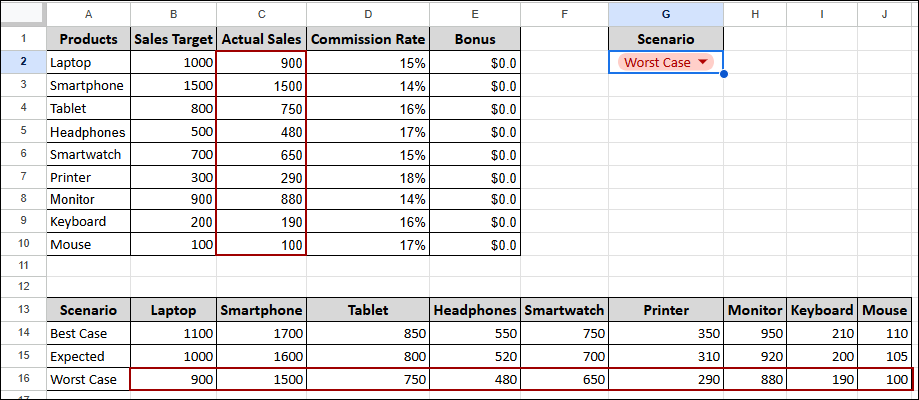
➤ Now, choose a scenario, Worst Case, from the drop-down menu.

Thus, column C will show the actual sales for the worst-case scenario. If the Best Case is selected, the values will change to the best-case figures.
This way, when you select a different scenario from the dropdown, the Actual Sales values in column C will automatically update to reflect that scenario.
Sensitivity Analysis in Google Sheets
Sensitivity analysis in Google Sheets helps you see how changes in one key variable affect your results. It’s a great way to understand the impact of things like cost, price, or profit margin on your overall outcome.
Suppose we have a dataset containing Product, Units Sold, Cost per Unit, and Profit Margin. In this section, we will calculate the Selling Price and Profit per Unit for each product, and then determine the Total Profit based on a specified profit margin.
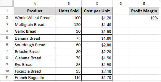
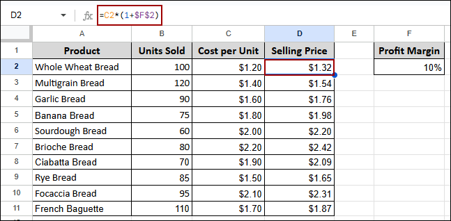
To calculate the Selling Price for each product using the Cost per Unit and the specified Profit Margin,
➤ Select cell D2 and enter the following formula.
=C2*(1+$F$2)
This formula multiplies the Cost per Unit by 1 plus the Profit Margin, which is locked with $ signs so it doesn’t change when copied.
Now, we will determine the profit per unit by subtracting the cost per unit from the selling Price and then multiplying by the units sold.
➤ Select a cell and enter the following formula.
=(D2-C2)*B2
This formula calculates the profit margin per unit and then multiplies it by the number of units sold.
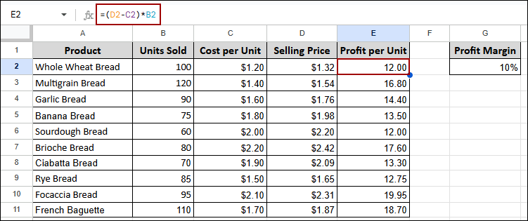
Finally, we will sum up all the profit per unit values to get the total profit.
➤ Select a cell and put the following formula.
=SUM(E2:E11)
This formula adds all the values in the Profit per Unit column from E2 to E11.
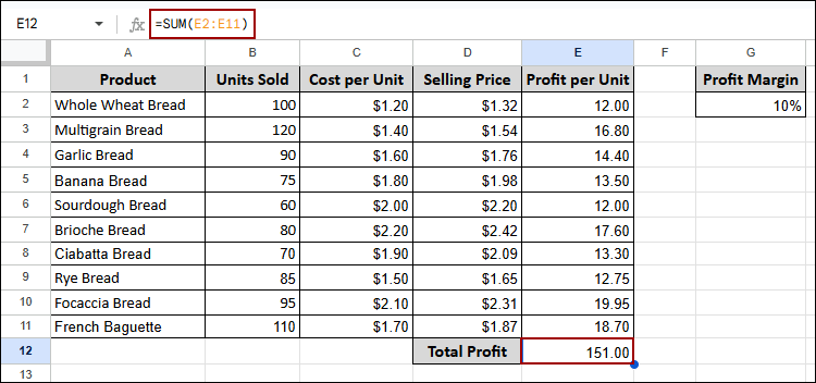
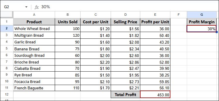
As a result, if we change the Profit Margin in cell G2 to 30%, the Selling Price, Profit per Unit, and consequently the Total Profit for all products will automatically update to reflect this higher margin. This demonstrates a sensitive analysis, showing how a change in one input significantly impacts the financial outputs of the entire product line.
What-If Analysis with Goal Seek in Google Sheets
In this method, we will use the Goal Seek add-on to set up a bonus calculation for a targeted value. Here, Google Sheets finds the exact sales needed to reach a specific bonus goal. This is a classic example of what if analysis, where you start with a desired outcome and work backward to find the necessary input.
Suppose we have a dataset containing: Products, Sales Target, Actual Sales, and Commission Rate. Now, we will use Goal Seek to find the exact sales needed to achieve a specific bonus amount based on these inputs.
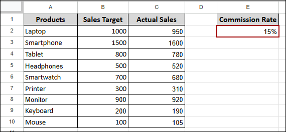
First, let’s set up a formula to calculate bonuses based on actual sales exceeding sales targets. To do so,
➤ Select a cell and enter the following formula.
=IF(C2>=B2, (C2-B2)*VALUE($F$2), 0)
This formula checks if Actual Sales are greater than the Sales Target. If true, it calculates the bonus as the excess sales multiplied by the commission rate; otherwise, the bonus is 0.
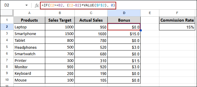
To determine what Actual Sales value is needed to achieve a specific bonus, we will use the Goal Seek add-on.
➤ To install the Goal Seek add-on, click Extensions > Add-ons > Get add-ons from the menu bar.
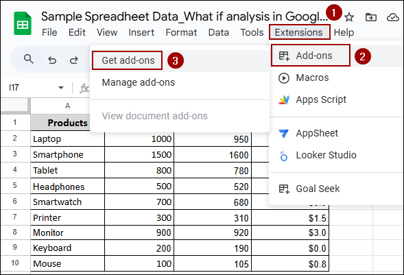
This will open the Google Workspace Marketplace.
➤ In the search bar, type Goal Seek and press Enter.
➤ Find Goal Seek for Sheets and click the Install button.
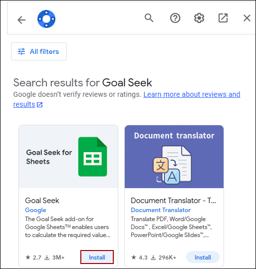
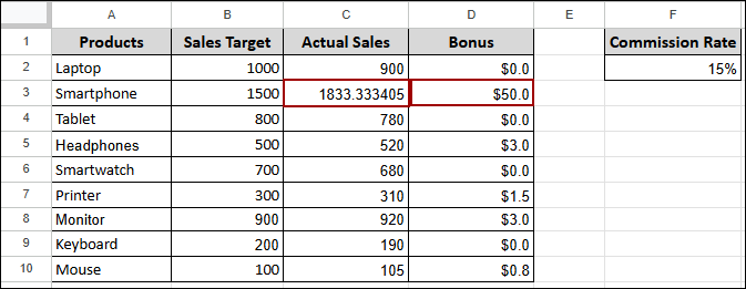
Once installed, you can use Goal Seek to find a target value. Let’s find out what Actual Sales are needed for the Smartphone to achieve a $50 bonus.
➤ Click Extensions > Goal Seek > Open from the menu bar.
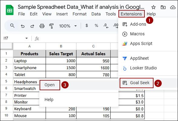
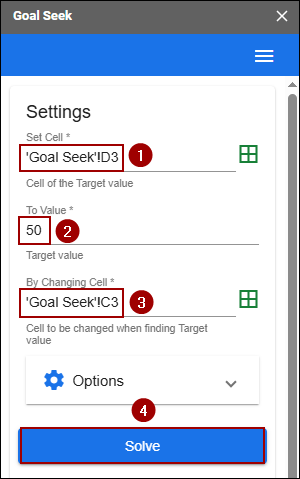
➤ In the Set Cell field, enter the cell that contains the formula you want to solve for (in this case, the Bonus cell for Smartphone).
➤ In the To Value field, enter your desired target value (50).
➤ In the By Changing Cell field, enter the cell that Goal Seek should adjust to reach the target (the Actual Sales cell for Smartphone).
➤ Finally, click Solve.
As a result, Goal Seek will calculate and display the Actual Sales value that is needed to achieve $50 bonus.
Frequently Asked Questions
Is there a built-in Scenario Manager in Google Sheets?
No, Google Sheets doesn’t have a built-in Scenario Manager like Excel, but you can create one manually using dropdowns and predefined input tables.
How do I know which variable has the biggest impact on results?
You can use sensitivity analysis to change one variable at a time and observe how your output changes; this shows which inputs matter most.
Can I visualize What-If results using charts?
Absolutely. Line charts, bar graphs, or even interactive dashboards can help you see the impact of different scenarios visually.
Concluding Words
Above, we’ve explored all the key methods to perform what-if analysis in Google Sheets, from manual inputs to Goal Seek and Sensitivity Analysis. These tools make it easy to test different scenarios, analyze outcomes, and make smarter decisions. Now you can confidently model, plan, and predict your data without needing complex tools. If you have any questions, feel free to drop them in the comment section below.
