The ARRAYFORMULA function in Google Sheets is handy when you want to apply a single formula for a large dataset. This function enables you to use a single formula across an entire range of cells or columns simultaneously. Thus, you don’t need to drag the formula manually. As it applies the formula to a range of whole columns, you might get errors for blank cells. In this article, we will provide a complete guide with formula examples and error-solving techniques for the ARRAYFORMULA function in Google Sheets.
Syntax of ARRAYFORMULA Function
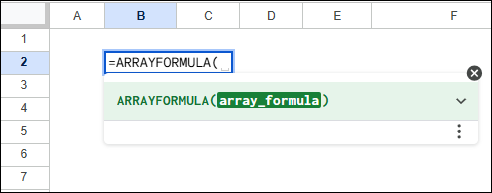
The syntax of the ARRAYFORMULA function works for the formula wrapped inside it.
=ARRAYFORMULA(array_formula)
array_formula: This part includes applying a formula across a range of cells or columns. The formula consists of functions such as IF, VLOOKUP, INDEX, and others, using array ranges (e.g., A2:A instead of A2).
ARRAYFORMULA Google Sheets Examples
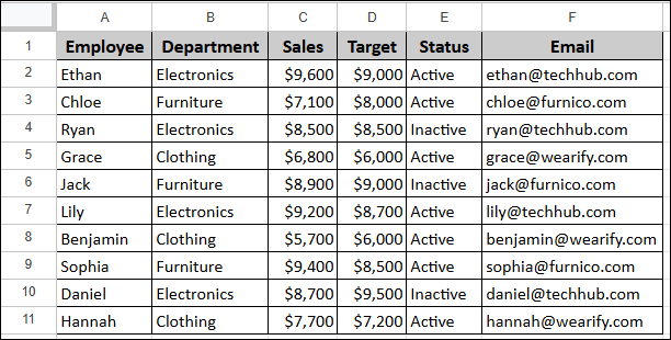
In this part, we will check out some examples of the ARRAYFORMULA function in Google Sheets. Suppose we have a sample dataset containing Employee, Department, Sales, Target, Status, and Email. Now, we will perform some calculations using the ARRAYFORMULA function.
Using ARRAYFORMULA Function for Automatic Calculation
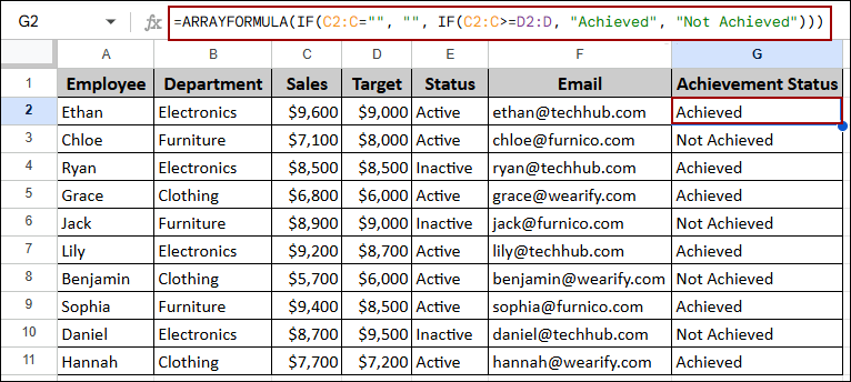
Traditionally, we used to apply a formula in one cell and then drag the formula across the column. But with the ARRAYFORMULA function, you won’t need to do it anymore. Here, we will use the ARRAYFORMULA function combined with the IF function to determine the Achievement status. We will apply a single formula for automatic calculation without dragging the Fill Handle.
➤ Select cell G2, write down the formula below, and press ENTER.
=ARRAYFORMULA(IF(C2:C="","", IF(C2:C>=D2:D, "Achieved", "Not Achieved")))
Formula Breakdown:
- IF (IF(C2:C=””,”” , …)): This part prevents the formula from processing blank rows. It returns an empty string (“”) if the Sales cell in column C is empty.
- IF (IF(C2:C>=D2:D, “Achieved”, “Not Achieved”)): This calculation is applied to all non-blank rows. It compares the entire Sales range (C2:C) against the Target range (D2:D) and provides text according to the condition.
- ARRAYFORMULA(…): This ensures the nested IF function processes the entire range, returning the calculated result (“Achieved” or “Not Achieved”) into the new column G.
As a result, we will get the correct conditional result for every employee in the Achievement Status column.
Applying Conditions with ARRAYFORMULA and IF Functions
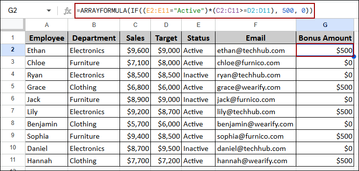
You can also apply different conditions combining ARRAYFORMULA and IF functions. Instead of a simple text status, we can use it to calculate a value based on multiple criteria. Here, we will calculate a Bonus Amount of $500 only if the conditions are true.
➤ Choose a cell G2, insert the following formula, and click ENTER.
=ARRAYFORMULA((IF(E2:E11="Active", 1, 0))*(C2:C11>D2:D11)*500)
Formula Breakdown:
- (IF(E2:E11=”Active”): Checks the first condition (Status is “Active”) and converts the result into 1 (TRUE) or 0 (FALSE).
- *(C2:C11>=D2:D11): Checks the second condition (Sales>=Target), which returns TRUE (1) or FALSE (0).
- *500: Multiplies the result of the two conditions by the bonus amount. The final result is $500 only if (1 * 1) occurs; otherwise, it is $0.
Thus, we can calculate the Bonus Amount for all employees by applying the “Active” and “Sales Met Target” conditions across all rows simultaneously.
Joining Numbers and Text
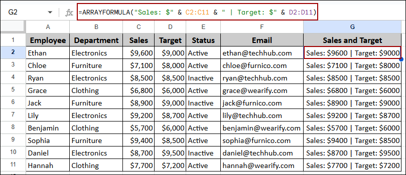
Using the ARRAYFORMULA function, you can also join text and numbers from multiple columns into a single text string for a range of cells. Here, we will create a column that combines the static text labels “Sales:” and “Target:” with numeric values from columns C and D for every employee.
➤ Select cell G2, enter the formula, and press ENTER.
=ARRAYFORMULA("Sales: $" & C2:C11 & " | Target: $" & D2:D11)
Formula Breakdown:
- ARRAYFORMULA(…): It ensures that the joining operation is done on the entire specified range, not just a single cell.
- “Sales: $” & C2:C11: Joins the static text “Sales: $” with the values found in the Sales range (C2:C11).
- ” | Target: $” & D2:D11: Joins the separator and the text ” | Target: $” with the values in the Target range (D2:D11).
As a result, we will get a text string in the Sales and Target column, joining the numeric values with text labels.
Google Sheets ARRAYFORMULA with INDEX and MATCH Functions
The INDEX and MATCH functions are mostly used for lookup tasks. Combining these functions with the ARRAYFORMULA, you can perform these lookups for an entire list of criteria at once. In this part, we will use these functions to extract specific data and pull data from another sheet.
Extracting Specific Data Using ARRAYFORMULA with INDEX and MATCH Functions
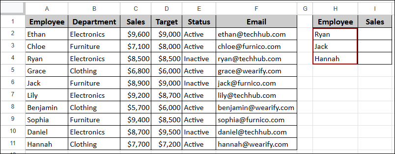
To extract specific data using ARRAYFORMULA with INDEX and MATCH functions, we will use the same dataset. Here, we will look up the Sales figures for a selected list of Employees listed in column H.
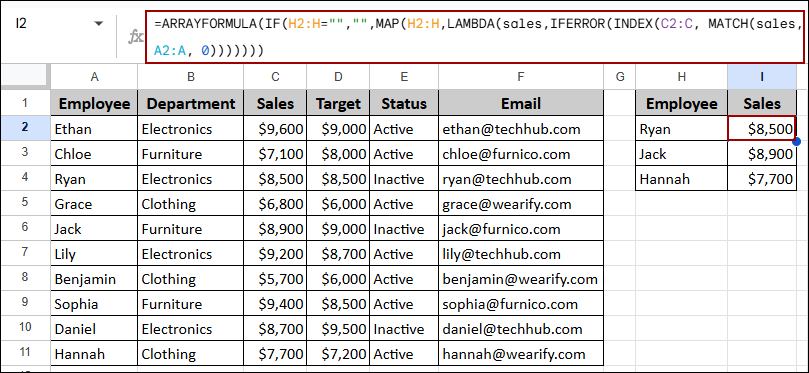
➤ Select the cell where you want the first result (I2), put the following formula, and hit ENTER.
=ARRAYFORMULA(IF(H2:H="","",MAP(H2:H,LAMBDA(sales,IFERROR(INDEX(C2:C,MATCH(sales,A2:A,0)))))))
Formula Breakdown:
- ARRAYFORMULA(…): This part is for applying this entire calculation across a range of cells.
- IF(H2:H=””,””,”…”: Checks if the Employee cells in Column H are blank. If they are, it returns a blank cell, preventing errors in unused rows.
- MAP(H2:H, LAMBDA(sales, …)): Repeats through every cell in the H2:H range, temporarily naming each value sales for processing.
- MATCH(sales, A2:A, 0): Finds the exact row number of the employee name (sales) within the Employee list (A2:A).
- INDEX(C2:C, …): Uses the row number returned by MATCH to retrieve the corresponding Sales value from the Sales column (C2:C).
- IFERROR(…): Handles cases where an employee name isn’t found, preventing the formula from returning an #N/A error.
Finally, the Sales column (I2:I4) will be filled with the correct figures corresponding to the employees listed in Column H.
Pulling Data from Another Sheet
The ARRAYFORMULA is a versatile function, allowing you to pull data from different sheets. Assume your main sheet is “Store A” and the employee sales data you need to pull from is on a sheet named “Store B”.
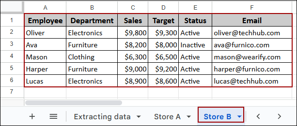
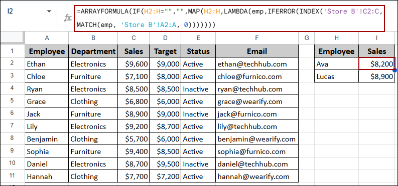
We will use the same structure as before to look up the Sales for “Ava” and “Lucas” from the “Store B” sheet. This time, the formula will refer to the external sheet name.
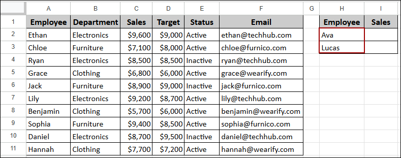
➤ In cell I2, write down this formula below and click ENTER.
=ARRAYFORMULA(IF(H2:H="","",MAP(H2:H,LAMBDA(emp,IFERROR(INDEX('Store B'!C2:C,MATCH(emp,'Store B'!A2:A,0)))))))
Formula Breakdown:
- ‘Store B’!C2:C and ‘Store B’!A2:A: This section references the Sales column and Employee column, on the sheet named ‘Store B’.
- MATCH(emp, ‘Store B’!A2:A, 0): Matches the employee name (emp) to the list in Store B’s Column A.
- INDEX(‘Store B’!C2:C, …): Returns the corresponding Sales value from Store B’s Column C.
Thus, we have successfully pulled the Sales data from the Store B sheet for the listed employees.
Concatenating Data Using ARRAFORMULA Function in Google Sheets
Concatenation is the process of joining or combining multiple text strings or cell values into a single cell. Using ARRAYFORMULA, this joining process is automatically applied to every row in the range. In this part, we will join text, conditional text and combine text and numbers with formatting.
Joining Text from Multiple Cells
Here, we will combine an employee’s name and their email address. We will use the ampersand operator (&) within ARRAYFORMULA to join texts across all rows.
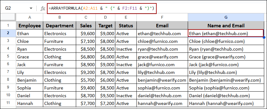
➤ Select cell G2, insert the formula, and press ENTER.
=ARRAYFORMULA(A2:A11 & " (" & F2:F11 & ")")
Formula Breakdown:
- ARRAYFORMULA(…): It applies the joining task for the entire range.
- A2:A11 & ” (” & F2:F11 & “)”: Concatenates the text in A2:A11 (Employee Name) with the literal string ” (“, then with the text in F2:F11 (Email), and finally with the literal string “)”.
Thus, the Name and Email column (G2:G11) now lists the employee’s name by their email address enclosed in parentheses.
Adding Conditional Text
Similarly, you can add conditional text for a range of cells using the ARRAYFORMULA with the IF function. Here, we will label employees based on their Sales and Target values.
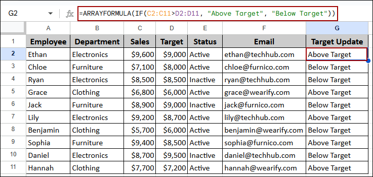
➤ Select cell G2, enter the following formula, and hit ENTER.
=ARRAYFORMULA(IF(C2:C11>D2:D11, "Above Target", "Below Target"))
Formula Breakdown:
- IF(C2:C11>D2:D11, “Above Target”, “Below Target”): It compares the Sales range (C2:C11) against the Target range (D2:D11). If a cell in C is greater than the corresponding cell in D, it returns “Above Target”; otherwise, it returns “Below Target”.
- ARRAYFORMULA(…): Ensures the IF statement is executed for every pair of cells in the specified ranges.
Finally, the Target Update column displays “Above Target” or “Below Target” for every employee row, based on the comparison of their sales (C) and target (D).
Combining Text and Numbers with Formatting
While joining text and currency/numerical data, you may lose the original formatting (like the dollar sign or decimal places). To get the proper output, you can use the TEXT function within ARRAYFORMULA. Here, we will combine the Employee Name with their achieved Sales amount, with the currency format.
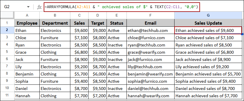
➤ In cell G2, write down the formula below, and hit ENTER.
=ARRAYFORMULA(A2:A11 & " achieved sales of $" & TEXT(C2:C11, "0,0"))
Formula Breakdown:
- TEXT(C2:C11, “0,0”): Converts the numerical sales data in C2:C11 into a text string using the specified format. The “0,0” format ensures a clean number without decimals but with a comma separator.
- A2:A11 & ” achieved sales of $” & …: Concatenates the Employee Name with the descriptive text and the formatted sales value.
- ARRAYFORMULA(…): It applies the joining and formatting to the entire range.
As a result, the output in the Sales Update column provides a formatted text summary for each employee, showing the Sales figures with the desired currency format.
Fixing ARRAYFORMULA Not Working in Google Sheets
The ARRAYFORMULA is really useful for a range of cells. But sometimes you will get errors when dealing with open-ended ranges or empty cells. When you get unexpected errors, it usually occurs due to blank rows and mismatched ranges. These errors can be fixed by wrapping the function with conditional logic.
Ignoring Blank Rows to Prevent Errors
While applying ARRAYFORMULA to a full column (e.g., C2:C) to process data, the formula will extend its output into blank rows. Thus, you will get errors or unnecessary output in the blank cells.
Problem:
To learn about this, we will use the same dataset as before, with some blank rows.
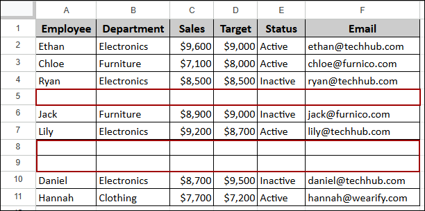
Now, let’s use a simple IF condition with ARRAYFORMULA to check if Sales met Target across a fixed range.
➤ Choose a cell, write down the formula, and click ENTER.
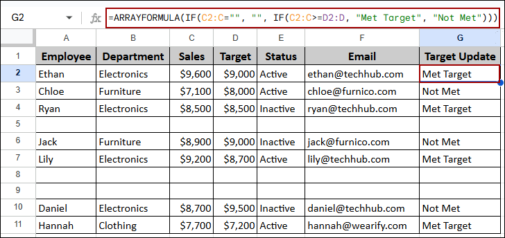
=ARRAYFORMULA(IF(C2:C11>=D2:D11, "Met Target", "Not Met"))
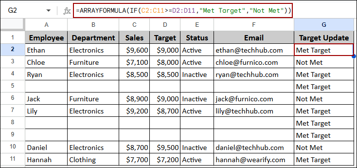
Thus, you will see that the blank rows return “Met Target” because the formula treats empty cells as the numeric value zero (0). As 0 is not less than 0, the formula qualifies with the condition, resulting in “Met Target” for those rows.
Solution:
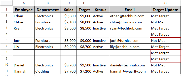
To solve this, we will use another IF condition that checks if the Sales cell (C2:C) is blank. Thus, it will return a blank result (“”) if it is empty.
➤ Select cell G2, put the correct formula, and hit ENTER.
=ARRAYFORMULA(IF(C2:C="", "", IF(C2:C>=D2:D, "Met Target", "Not Met")))
This way, the formula returns the correct result only for rows that contain data in the Sales column (C), leaving the remaining rows blank.
Fixing Mismatched Range Size Problems
While using the ARRAYFORMULA function, you must ensure all ranges involved in a calculation have the same number of rows or columns. If mismatched ranges are inserted, the function often returns a #N/A error.
Problem:
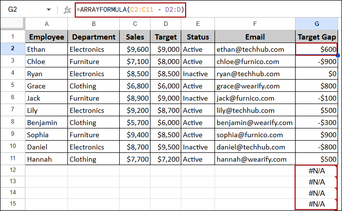
To describe this, let’s calculate the Target Gap. For this, we will use a mismatched range: a defined range for Sales (C2:C11) and an open-ended range for Target (D2:D).
➤ Choose a cell, write down the formula, and click ENTER.
=ARRAYFORMULA(C2:C11 - D2:D)
Here, you will see the limited range of C2:C11 conflicts with the open-ended range of D2:D, resulting in the #N/A error in the rows.
Solution:
To solve this, you must ensure that all ranges in the calculation are consistent.
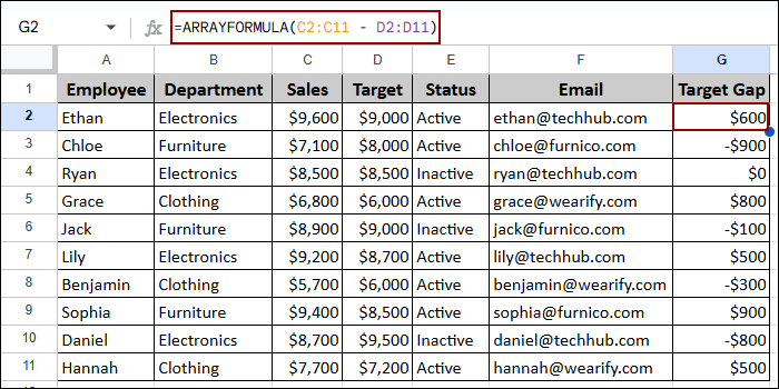
➤ Select cell G2, put the correct formula, and hit ENTER.
=ARRAYFORMULA(C2:C - D2:D)
This way, by making all ranges open-ended, the formula applies the subtraction to all corresponding rows, ignoring the #N/A error.
Handling #DIV/0! Errors for Empty Cells Using IFERROR Function
Sometimes you will get #DIV/0! Error in blank cells if the formula involves division. This happens because division by zero is mathematically undefined, showing #DIV/0! Error in blank cells.
Problem:
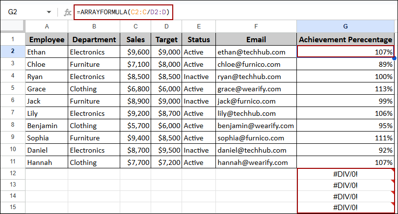
Let’s calculate the Achievement Percentage (Sales divided by Target) using open-ended ranges.
➤ Choose a cell, write down the formula, and click ENTER.
=ARRAYFORMULA(C2:C/D2:D)
Thus, you will get the #DIV/0! Error for the blank cells as the formula applies the division to rows where both the Sales (C) and Target (D) cells are blank.
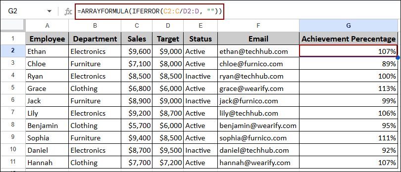
Solution:
To solve this, we will use the IFERROR function to ignore errors.
➤ Select cell G2, put the correct formula, and hit ENTER.
=ARRAYFORMULA(IFERROR(C2:C/D2:D, ""))
This way, the formula calculates the Achievement Percentage correctly for all data rows. The IFERROR function returns a blank where any division error is found.
Frequently Asked Questions
Why is ARRAYFORMULA not calculating dates correctly?
This happens when text is mixed with date values. Ensure the date column is formatted as Date, and the formula references the entire column.
Why do I get #REF! Error while using ARRAYFORMULA with JOIN?
The JOIN function cannot output row-by-row results. You can use the TEXTJOIN function for a single combined output, or the BYROW function for row-wise joining.
Why does ARRAYFORMULA double my results when sorting the sheet?
Sorting can misalign referenced columns. For this, you can convert formulas to use dynamic references like the INDEX function instead of fixed row numbers.
Concluding Words
Above, we have covered a complete guide to the ARRAYFORMULA function in Google Sheets. By using this function, you can process entire ranges with a single formula. Combining these with INDEX and MATCH functions, you can extract data from a list or another sheet. We also discussed troubleshooting problems and solutions, such as using the IF function to handle blank rows and the IFERROR function to manage division errors. If you have any queries, feel free to share them in the comment section below.