The SUMIF function in Google Sheets is used for summing values based on specific criteria. Whether you need to sum values based on text matches, dates, multiple conditions, or even cell colors, the SUMIF function can simplify the calculations. In this article, we will provide a complete guide with formula examples and step-by-step instructions for the SUMIF function in Google Sheets.
Syntax of SUMIF Function in Google Sheets
The SUMIF function adds up values in a range that meet a single criterion.
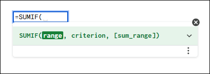
=SUMIF(range, criterion, [sum_range])
- range: The range of cells you want to evaluate against the criterion.
- criterion: The condition that determines which cells to include in the sum. This can be a number, text, cell reference, or an expression.
- sum_range: (Optional) The actual cells to sum. If omitted, the function sums the cells in the range.
Using SUMIF Function with Text Criteria in Google Sheets
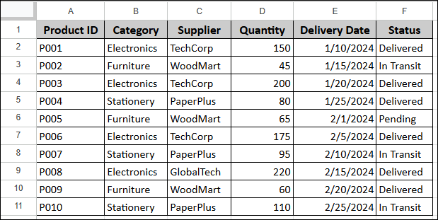
In this section, we will explore how to use the SUMIF function with various text criteria. Suppose we have a sample dataset containing Product ID, Category, Supplier, Quantity, Delivery Date, and Status columns.
Summing Values When Cell Contains Specific Text
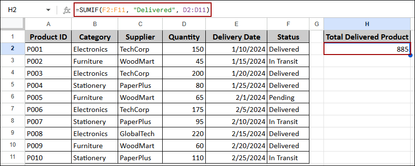
You can use the SUMIF function to sum values when cells contain an exact text match. Here, we will calculate the total quantity of products that have been “Delivered”.
➤ Select cell H2, write down the formula below, and press ENTER.
=SUMIF(F2:F11, "Delivered", D2:D11)
Formula Breakdown:
- F2:F11: The range of cells in the Status column that we want to evaluate.
- “Delivered”: The exact text criterion we are looking for.
- D2:D11: The range of cells in the Quantity column to sum.
- SUMIF(…): Adds up all quantities where the status matches “Delivered”.
As a result, the formula returns 885, indicating the total quantity of delivered products.
Summing Values with Partial Text Matches
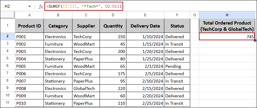
You can also sum values when cells contain partial text using wildcard characters. The asterisk (*) sign represents any number of characters. Here, we will calculate the total quantity ordered from suppliers whose names contain “Tech”.
➤ Select cell H2, insert the following formula, and click ENTER.
=SUMIF(C2:C11, "*Tech*", D2:D11)
Formula Breakdown:
- C2:C11: The range of cells in the Supplier column.
- “*Tech*”: The wildcard criterion that matches any cell containing “Tech” anywhere in the text.
- D2:D11: The range containing the quantities to sum.
- SUMIF(…): Adds up all quantities where the supplier name contains “Tech”.
Thus, the formula returns 745, showing the total quantity ordered from TechCorp and GlobalTech combined.
Summing Based on Text in Another Column
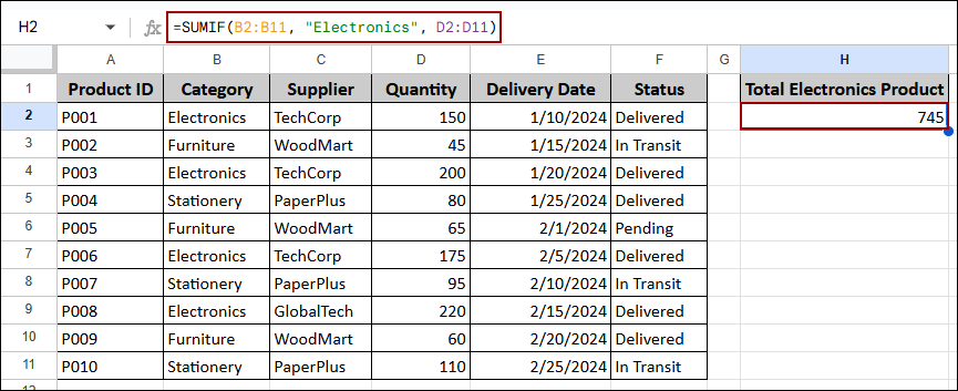
Sometimes you need to sum values based on criteria in one column while summing values from another column. Here, we will calculate the total quantity of all “Electronics” products.
➤ Choose cell H2, enter the formula, and hit ENTER.
=SUMIF(B2:B11, "Electronics", D2:D11)
Formula Breakdown:
- B2:B11: The range we are evaluating in the Category column.
- “Electronics”: The criterion that matches products in the Electronics category.
- D2:D11: The range containing the quantities to sum.
- SUMIF(…): Adds up all quantities where the category is “Electronics”.
As a result, the formula returns 745, representing the total quantity of electronics products.
Summing Values Not Equal to Specific Value
You can sum values that do not match a specific criterion by using the not equal to operator (<>). Here, we will calculate the total quantity of products that are not “Delivered”.
➤ Choose cell H2, write down the formula, and press ENTER.
=SUMIF(F2:F11, "<>Delivered", D2:D11)
Formula Breakdown:
- F2:F11: The range we are checking in the Status column.
- “<>Delivered”: The criterion that matches any value not equal to “Delivered”.
- D2:D11: The range containing the quantities to sum.
- SUMIF(…): Adds up all quantities where the status is not “Delivered”.
Thus, the formula returns 315, showing the total quantity of products that are either “In Transit” or “Pending”.

Using SUMIF Function for Non-Blank Cells
The SUMIF function is useful for summing values only when cells are not empty. This helps you calculate totals while excluding rows with missing data. Suppose we have the same dataset with some blank cells in the Supplier column.
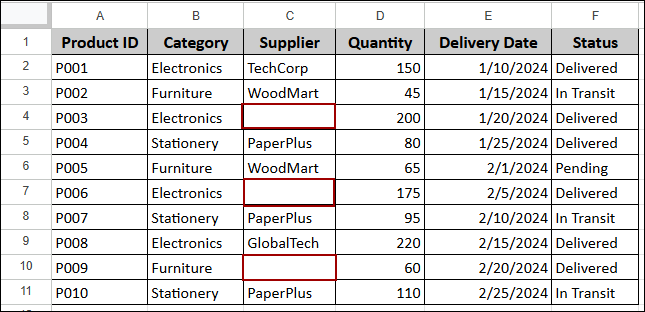
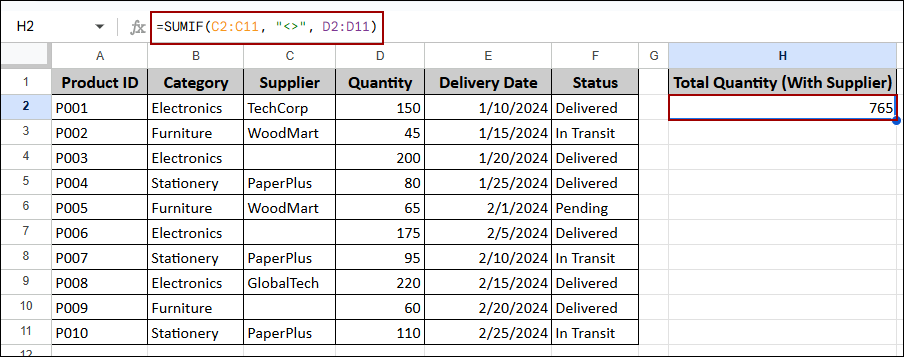
To sum quantities only for products that have a supplier listed, you can use the not equal to blank criterion. Here, we will calculate the total quantity of products with an assigned supplier.
➤ Select cell H2, write down the formula below, and press ENTER.
=SUMIF(C2:C11, "<>", D2:D11)
Formula Breakdown:
- C2:C11: The range of cells in the Supplier column.
- “<>”: The criterion that matches any non-blank cell.
- D2:D11: The range containing the quantities to sum.
- SUMIF(…): Adds up all quantities where the supplier cell is not empty.
As a result, the formula returns 765, indicating the total quantity of products with a supplier assigned.
Google Sheets SUMIF Function with Multiple Criteria
When you need to sum based on multiple conditions simultaneously, you can use the SUMIFS function instead of the SUMIF function. Here, we will calculate the total quantity of “Furniture” products that have been “Delivered”.
➤ Choose cell H2, write down the formula, and press ENTER.
=SUMIFS(D2:D11, B2:B11, "Furniture", F2:F11, "Delivered")
Formula Breakdown:
- D2:D11: The range containing the values to sum (Quantity column).
- B2:B11, “Furniture”: The first criterion checks if the Category is “Furniture”.
- F2:F11, “Delivered”: The second criterion checks if the Status is “Delivered”.
- SUMIFS(…): Adds up quantities that meet both criteria simultaneously.
Thus, the formula returns 60, showing that the total quantity of delivered furniture products is 60.

Summing Values Based on Date Range
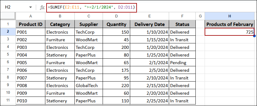
The SUMIF function can be used to sum values based on date criteria using comparison operators. Here, we will calculate the total quantity of products with delivery dates in February 2024 or later.
➤ Select cell H2, enter the following formula, and hit ENTER.
=SUMIF(E2:E11, ">=2/1/2024", D2:D11)
Formula Breakdown:
- E2:E11: The range of cells in the Delivery Date column.
- “>=2/1/2024”: The criterion that checks if dates are on or after February 1, 2024.
- D2:D11: The range containing the quantities to sum.
- SUMIF(…): Adds up all quantities where the delivery date meets the condition.
As a result, the formula returns 725, indicating the total quantity of products scheduled for delivery in February 2024 or later.
Using SUMIF Function for Summing Data from Another Sheet
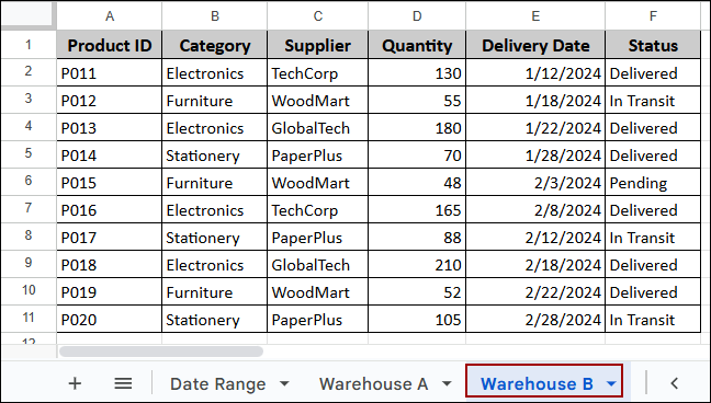
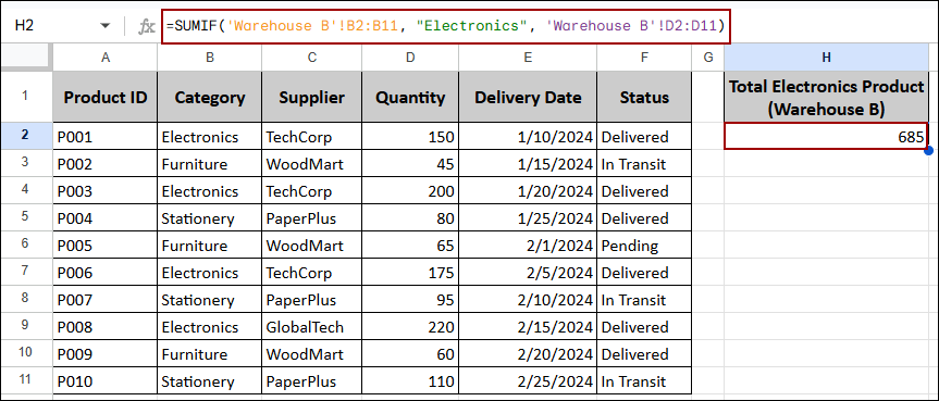
You can use the SUMIF function to sum data from a different sheet within the same workbook. Suppose we have some more data in a sheet named “Warehouse B”. Here, we will calculate the total quantity of “Electronics” products from Warehouse B in another sheet.
➤ Choose cell H2, insert the formula, and click ENTER.
=SUMIF('Warehouse B'!B2:B11, "Electronics", 'Warehouse B'!D2:D11)
Formula Breakdown:
- ‘Warehouse B’!B2:B11: The range in the Category column from the Warehouse B sheet.
- “Electronics”: The criterion that matches products in the Electronics category.
- ‘Warehouse B’!D2:D11: The range containing the quantities to sum from Warehouse B.
- SUMIF(…): Adds up all electronics quantities from the specified sheet.
Thus, the formula returns 685, showing the total quantity of electronics products in Warehouse B.
Summing Cells by Color in Google Sheets
Google Sheets does not have a built-in function to sum cells by color, but you can create a custom function using Apps Script. Suppose we have the same dataset containing some colored cells in the Status column. Here, we will sum quantities for products with a specific background color in the Status column.

➤ Click on Extensions in the menu bar, then select Apps Script.

➤ In the Apps Script editor, paste the following script and click Run.
function sumByColor(sumRange, colorRange, color) {
var sheet = SpreadsheetApp.getActiveSpreadsheet();
var sumRangeData = sheet.getRange(sumRange);
var colorRangeData = sheet.getRange(colorRange);
var sumValues = sumRangeData.getValues();
var bgColors = colorRangeData.getBackgrounds();
var total = 0;
for (var i = 0; i < bgColors.length; i++) {
for (var j = 0; j < bgColors[0].length; j++) {
if (bgColors[i][j] == color) {
total += sumValues[i][j];
}
}
}
return total;
}
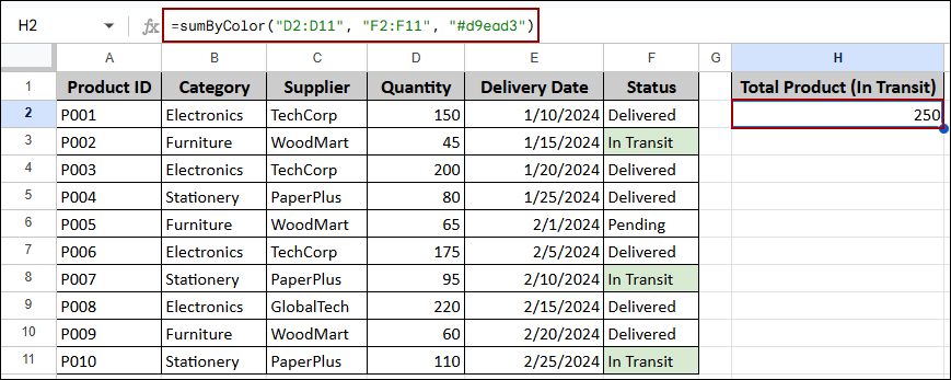
Now you can use this custom function in the sheet. Here, we will sum quantities for products with a light green background color (hex code #d9ead3) in the Status column.
➤ Select cell H2, enter the formula, and press ENTER.
=sumByColor("D2:D11", "F2:F11", "#d9ead3")
Formula Breakdown:
- “D2:D11”: The range of cells containing the values to sum (Quantity column).
- “F2:F11”: The range of cells to check for colored backgrounds (Status column).
- “#d9ead3”: The hex color code of the background color you want to match.
- sumByColor(…): The custom function that loops through the color range and sums matching values.
As a result, the formula returns 250, showing the total quantity of products with the specified background color in their status.
Frequently Asked Questions
Why does SUMIF function return 0 when summing based on dates?
This usually happens due to date formatting issues. Ensure both the criterion and the range are formatted as dates. Use the DATE function in your criterion or reference a cell containing the date instead of typing it directly as text.
Can SUMIF function work with multiple sum ranges?
No, the SUMIF function can only sum one range at a time. If you need to sum multiple ranges with the same criterion, you can add multiple SUMIF functions together or use array formulas to combine the results.
How do I use SUMIF with “greater than” or “less than” criteria?
Use comparison operators in quotes with the criterion. For example, “>100” for values greater than 100, “<50” for values less than 50, or “>=75” for values greater than or equal to 75.
Concluding Words
Above, we have covered a complete guide to the SUMIF function in Google Sheets. By using this function, you can sum values based on various criteria including text matches, partial matches, date comparisons, multiple conditions, and data from other sheets. We also explored how to sum non-blank cells, create custom functions for summing by color, and work with different types of criteria. If you have any queries, feel free to share them in the comment section below.
