When you are entering data in your Google Spreadsheet, dropdown menus can speed up and increase the accuracy of your data. You don’t need to enter values manually. Using a dropdown, you can select the pre-made list of data. Dropdown makes your sheet well organized and prevents typing errors.
What Is a Dropdown List in Google Sheets?
A dropdown menu is a feature in Google Sheets that allows you to select a value from a pre-specified list of possibilities inside a cell. You don’t need to input anything manually. Clicking the small arrow in the cell allows you to choose an item from the list.
It helps with:
- Faster input of data
- Avoiding Spelling Mistakes or inconsistent values
- Maintaining a readable spreadsheet.
Creating and Editing a Dropdown List in Google Sheets
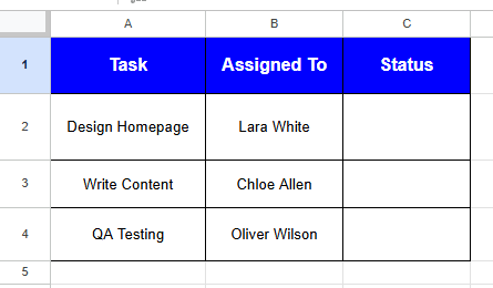
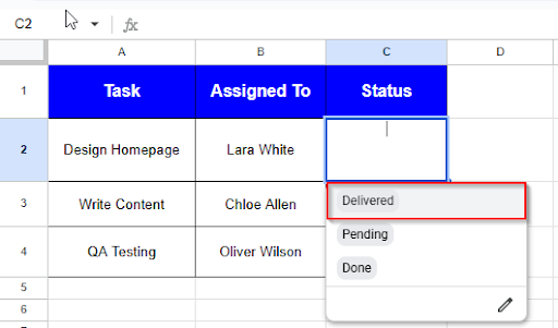
Drop-down lists help maintain data organization and provide error-free data easily. When you are working with repeating data, you can select data from a fixed list of options. Let’s look at the “Task List” dataset below, where you can see the process of creating and editing a dropdown list in Google Sheets.
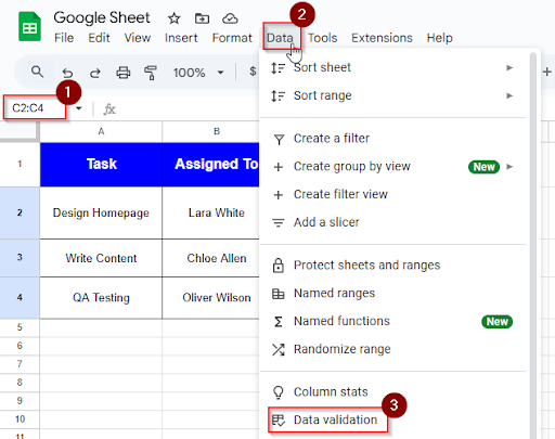
➤ Select the Cells C2: C4
➤ Click Data → Data validation
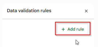
➤ Click on “+ Add rule”
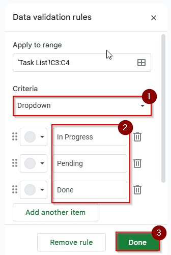
➤ Choose “Dropdown“
➤Enter your options, separated by commas: To Do, In Progress, Done and click “Done”
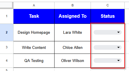
➤ Your dropdown list is created in cells C2:C4
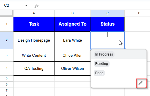
➤ Click on cell C2 and then click on the edit icon to edit the drop-down list.
➤ Edit your list and click Done.
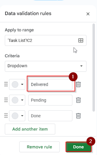
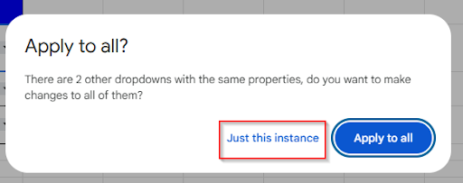
➤ Click on the “ Just this instance” option to apply this edit in the C2 cell only.
➤ Now you can see that the first instance is edited successfully.
Creating Multiple Dependent Dropdown Lists from Another Sheet in Google Sheets
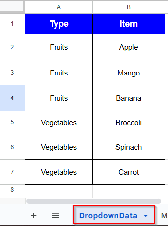
You can display a second dropdown list with dependent dropdowns. A dependent dropdown changes according to the first choice list. When you want to display related options, such as categories and subcategories, a multiple dependent dropdown is helpful. Let’s examine the dataset below, which consists of two sheets: the main sheet and the “DropdownData” sheet. Now we’ll create the drop down list based on the data from another sheet.
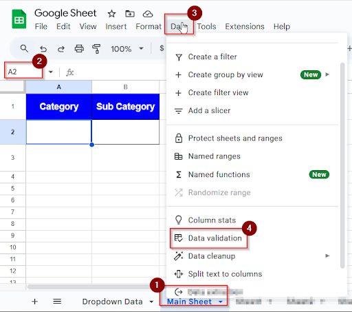
➤ In the “ Main Sheet”, select cell A2 and click Data, then Data Validation.
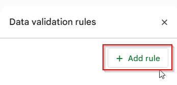
➤ Click on the “Add rule” option.
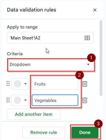
➤ Select Criteria “ Dropdown”, then type the options Fruits and Vegetables and click Done.
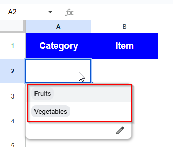
➤ In cell A2, you can see the drop-down list
➤ Type this formula in cell B2:
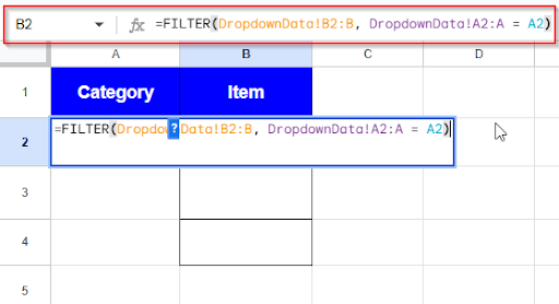
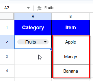
➤ Now you can see the result. If you select Fruits in A2, you can see the fruit list in B2. If you select vegetables in cell A2, you can see the vegetable items in the list.
Updating Cell Values Based on a Selection in a Dropdown List in Google Sheets
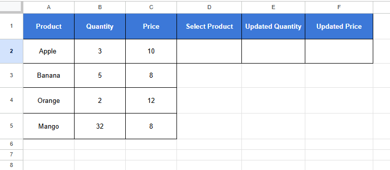
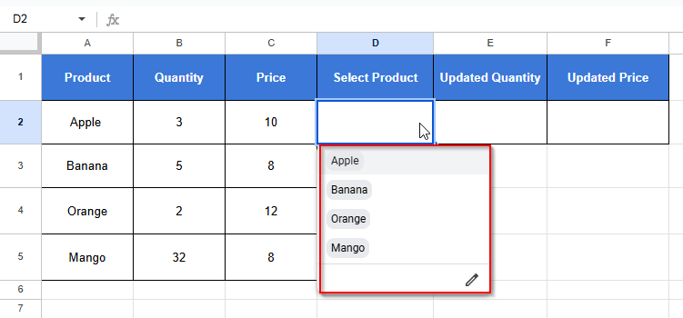
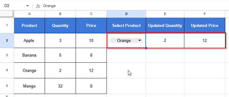
When a user selects a value from a drop-down list, the cell values will automatically be updated. This is a useful way to maintain Forms, inventory systems, and dashboards. Let’s look at the dataset below, where you want to update the Quantity and Price for that product based on the user’s selection. We’ll learn here updating the cell values based on a selection in the drop down list.
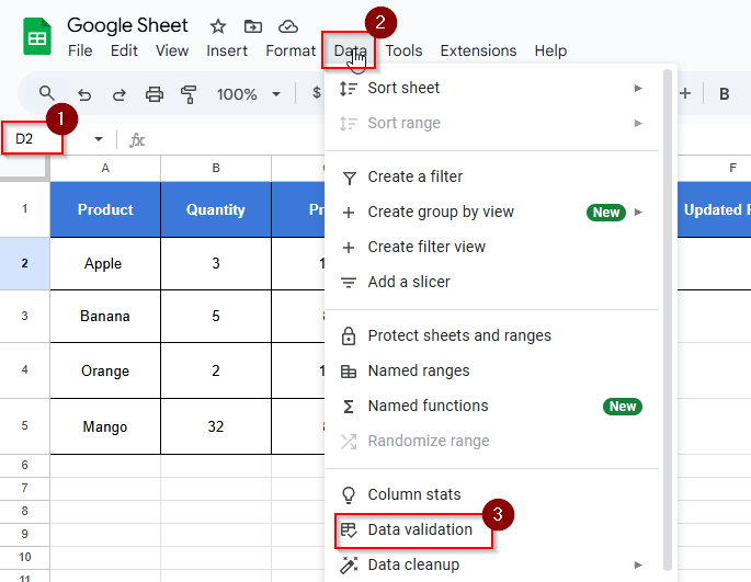
➤ Click on cell D2
➤ Go to Data → Data Validation.
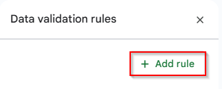
➤ Click the “Add rule” option.
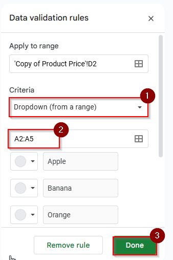
➤ Set Criteria to: “Dropdown from a range”, and choose A2:A5, then click Done.
➤ You can see the product list in cell D2
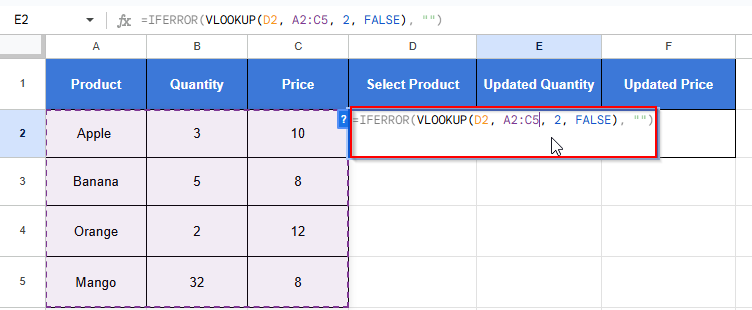
➤ Type the formula in the E2 cell for the updated Quantity:
➤ Type the formula in the F2 cell for the updated price :
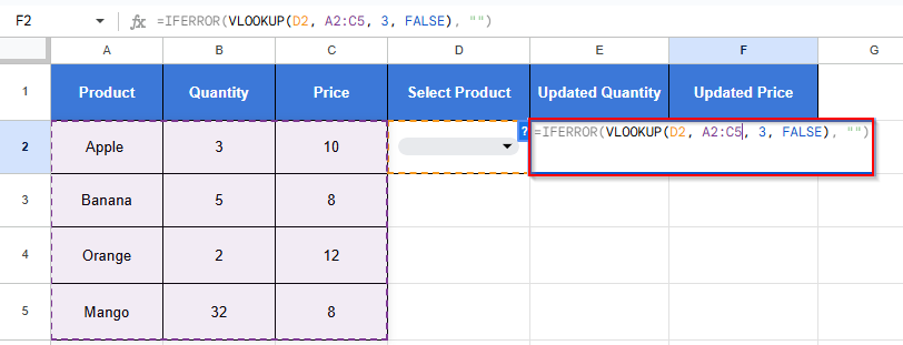
➤ Now you can see the result. If you select orange in the D2 cell, you can see the Quantity and Price of the orange.
Counting Dropdown Items in Google Sheets
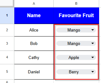
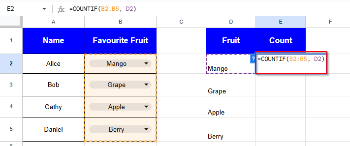
When you want to count the dropdown items in Google Sheets, you can do it using the COUNTIF function. This is helpful for task trackers, order forms, and surveys. Let’s look at the dataset below, where you can count how many times each fruit has been selected from the dropdown.
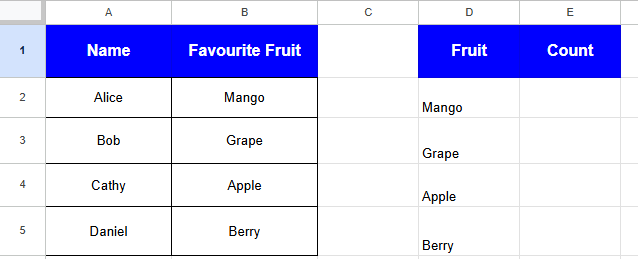
➤ Select cell B2:B5, Data> Data Validation

➤ Select the “Dropdown” Criteria and click DONE
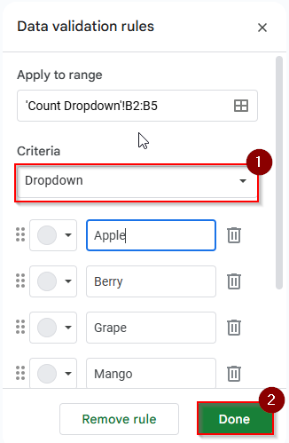
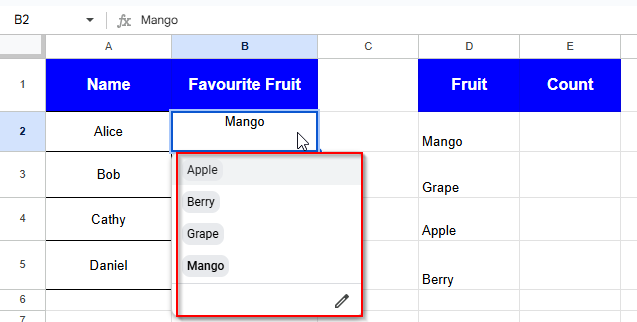
➤ Now you can see the fruit name list in B2: B5
➤ Write the formula in the E2 cell
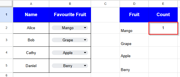
➤ Press Enter and see the result in cell E2
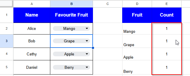
➤ Drag the formula down to see other cells.
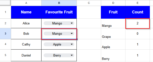
➤ If I select “Mango” in cell B3, then in cell E2, you can see the result is 2
Creating a Calendar Dropdown in Google Sheets
A Date picker is known as a calendar dropdown in Google Sheets. Without any error, you can choose dates more quickly by using date pickers. This is a useful method where users must enter dates regularly for booking schedules or working in an attendance sheet. Let’s look at the dataset below, where we’ll make a calendar-style dropdown in the “Date of Visit” column.
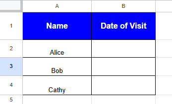
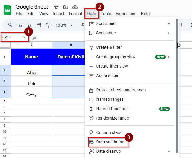
➤ Select B2:B4 cells and click Data> Data Validation
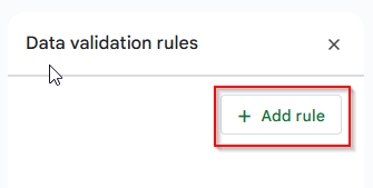
➤ Click the + Add rule option.
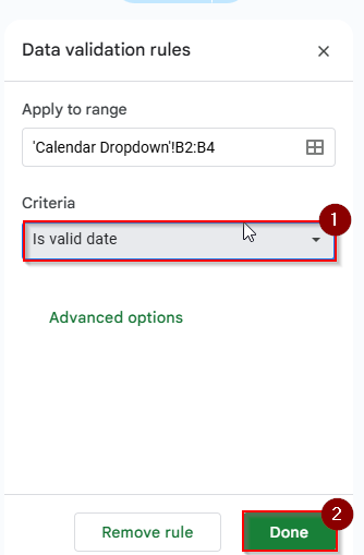
➤ Select the criteria “ is valid date” and click Done
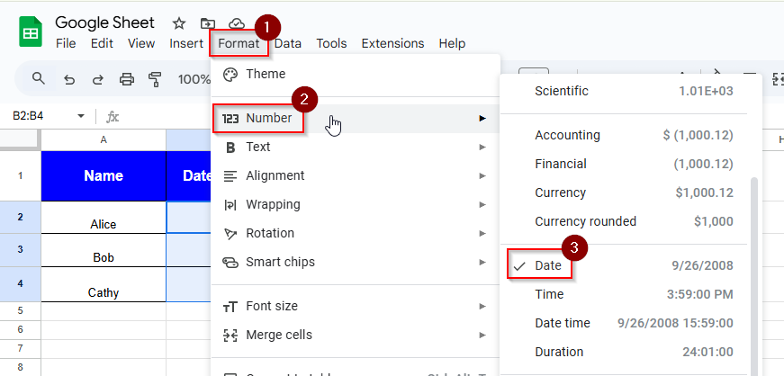
➤ Select the B2:B4 cells and click Format> Number>Date
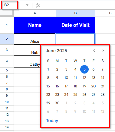
➤ Double click in the B2 cell to see the dropdown calendar
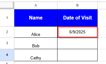
➤ The selected date will show in the B2 cell
Frequently Asked Questions
Is it possible to give a warning to the user if someone enters a value that is not in the menu?
Of Course. Select either the “Show warning” or “Reject input” option under Data Validation.
How many things can be in a dropdown menu?
Normally, it’s thousands of options in a dropdown menu, but for performance, it’s better to stay within 100–500. But you can use the Sheet Range option rather than manual typing.
What could be wrong with my dropdown menu?
If the dropdown is not working properly, then check the data validation conditions, range of sources is removed or not and the cell format. If you are using the mobile app, then the dropdown feature will not work properly.
Concluding Words
To maintain data accuracy, organization and usability, dropdown menus are a great method in Google Sheets. Dropdown menus help make schedules, forms, dashboards, or trackers. You can save time and reduce errors by using a dropdown in Google Sheets.