Google Sheets is a powerful tool for collaboration and data organization. Sometimes, you can see that your data isn’t updated when you are working with formulas, scripts, or other data connections. At that time, you need to refresh Google Sheets. In this article, I will describe how to refresh Google Sheets in many ways, from simple manual refresh to automated data updates.
Refreshing Formula in Google Sheets Automatically
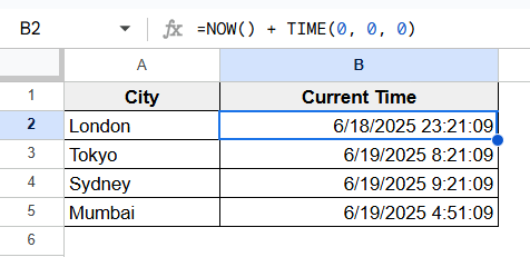
When working with dashboards or real-time data, you may feel frustrated when the formulas fail to refresh. You can use dynamic functions like IMPORTRANGE, GOOGLEFINANCE, and NOW to update formulas automatically. You need to set the option “on change and every minute” to refresh your sheet every minute.
Look at the dataset below, where we have used the NOW function to refresh the current time automatically.
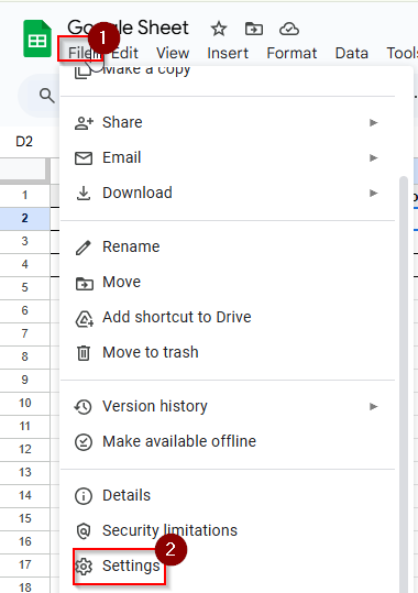
➤ Go to File > Settings
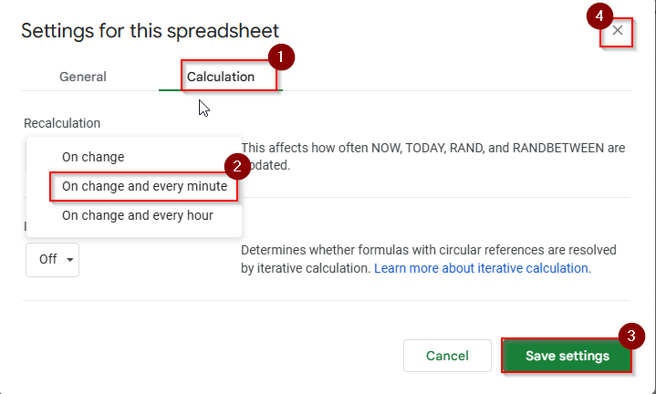
➤ Go to the Calculation tab
➤ Under Recalculation, choose “On change and every minute“
➤ Click Save Settings and close the pop-up.
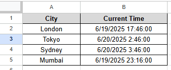
➤ Now you can see that the current time is changing every minute. The entire sheet is refreshed with formulas automatically.

Refreshing Google Sheets Using a Button
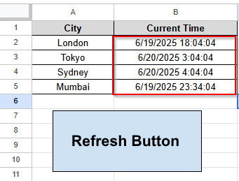
Google Sheets doesn’t have a “Refresh” button to refresh your sheet automatically, but you can make your own button. When you press that button, it will refresh your sheet. Using Apps Script, you can create a button to refresh your sheet. Let’s look at the dataset first, where the city names and current times of those cities are there. We need to refresh this current time using the refresh button.
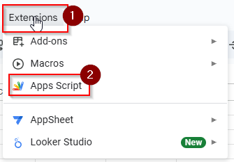
➤ Click Extensions > Apps Script option to write code for the refresh button.
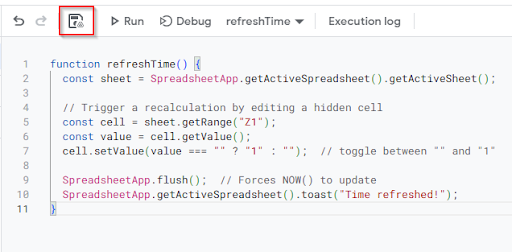
➤ Write the following code in the Apps Script area.
function refreshTime() {
  const sheet = SpreadsheetApp.getActiveSpreadsheet().getActiveSheet();
  // Trigger a recalculation by editing a hidden cell
  const cell = sheet.getRange("Z1");
  const value = cell.getValue();
  cell.setValue(value === "" ? "1" : "");  // toggle between "" and "1"
  SpreadsheetApp.flush();  // Forces NOW() to update
  SpreadsheetApp.getActiveSpreadsheet().toast("Time refreshed!");
}
➤ Click on the save option to save this code.
➤ Go to Insert > Drawing to make a refresh button
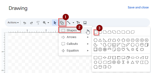
➤ In the drawing section, click in the circle> Shapes> Rectangle
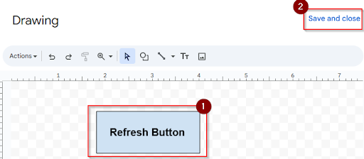
➤ Draw a rectangle and write “Refresh Button”, then click Save and Close
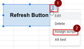
➤ Right click on that button, click the three dots option, and then “Assign Script”
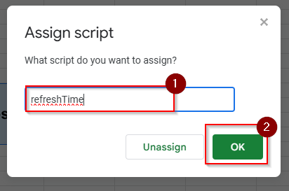
➤ Write “refreshTime” in the Assign Script menu and click OK. The refresh button will work now.
➤ Before clicking the refresh button, observe the current time of those cities
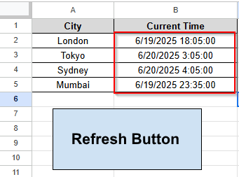
➤ Now you can see that, after clicking the refresh button, the current time is changed and refreshed.
Refreshing Pivot Table in Google Sheets
When you are working with big datasets, you can use a pivot table to summarize your data in Google Sheets. But when you are changing the main dataset, your Pivot Table will not always update immediately. You need to add the new cell range to the pivot table, and then the pivot table will be updated with the new data.
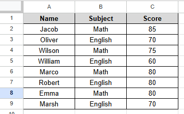
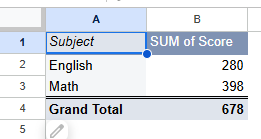
Let’s look at the dataset below, where we will see the sum of scores in the pivot table. We will add a new row to that table, and then add that cell range to the pivot table to refresh the table and get the updated scores.
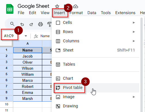
➤ Select cells (A1:C9)
➤ Go to Insert > Pivot table
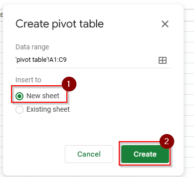
➤ Choose to insert in a New Sheet, and the pivot table will show in a new sheet.
➤ In the Pivot Table editor, find the Rows option and Add Subject.
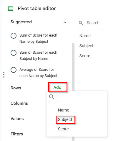
➤ In the Values option, Add Score
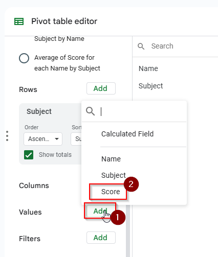
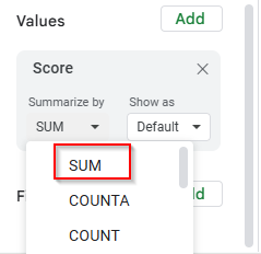
➤ Then set to SUM
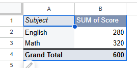
➤ Now you can see the average score of row A1:C9 in the pivot table.
➤ In the main dataset, add new data in row 10
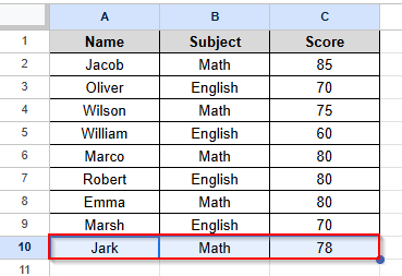
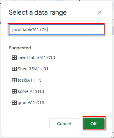
➤ Select the new data in a data range A1:C10 and click OK to see the updated pivot table.
➤ Now you can see the pivot table refreshes with new data.
Frequently Asked Questions
How to refresh formulas automatically once every minute?
Select the following: File > Settings > Calculation > Recalculation, and then set “On change and every minute”
Why does Google request permission in Apps Script?
When you have written custom scripts in App Scripts, these scripts are considered unverified. That’s why Google requires verification of your scripts and asks permission. Select your Google account and click the “Allow” option to give permission. You have to do this once to verify this script.
Concluding Words
When you are working with dynamic formulas and a pivot table, you need to refresh your data frequently. There is an easy option in Google Sheets to stay up to date, whether you are using the built-in settings or a custom refresh button.