In Excel, summing values based on whether they fall between two cell-defined limits is an effective way to analyze data, especially when working with price, quantity, sales, or any other numeric ranges. Whether you’re filtering data between thresholds or excluding a specific value altogether, Excel offers multiple flexible formulas to get the result you need.
In this article, we’ll explore various ways to sum values that are greater than and less than a cell value, including methods that use functions like SUMIF and SUMIFS, dynamic ranges, and structured references. We’ll also learn how to handle cases where you need to exclude a specific value, use constants, or create formulas that update automatically with your dataset. Let’s get started.
Steps to sum if greater than and less than cell value in Excel:
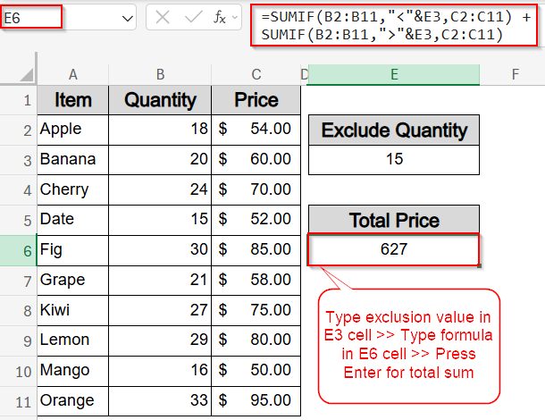
➤ Type your exclusion value such as 15 in cell E3.
➤ Click a blank cell like E6 to enter your formula.
➤ Type this formula to sum values that are less than or greater than the reference cell:
=SUMIF(B2:B11,”<“&E5,C2:C11) + SUMIF(B2:B11,”>”&E5,C2:C11)
Here, B2:B11 is the quantity column, C2:C11 is the price column, and E5 contains the value to skip.
➤ Press Enter to see sum results.
Exclude a Specific Value Using SUMIF Function Greater Than and Less Than a Cell
This method helps sum values by explicitly excluding a specific number in a referenced cell. It uses two SUMIF functions, one to capture values below the cell and another for those above it. You can also use SUMIFS with the <> operator as an alternative approach. For example, if you want to exclude quantities equal to 15 and only include prices where the quantity is greater than or less than 15, this method will return the correct sum. It’s a reliable technique when you want to ignore a specific threshold while still considering values on either side.
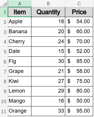
We’ll use the following dataset with Item names in column A, Quantity in column B and Price in column C to find the total sum with set criteria:
Steps:
➤ Type your exclusion value such as 15 in cell E3.
➤ Click a blank cell like E6 to enter your formula.
➤ Type this formula to sum values that are less than or greater than the reference cell:
=SUMIF(B2:B11,”<“&E5,C2:C11) + SUMIF(B2:B11,”>”&E5,C2:C11)
Here, B2:B11 is the quantity column, C2:C11 is the price column, and E3 contains the value to skip.
➤ Press Enter.
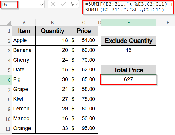
The result will be the total of all prices except where the quantity equals 15.
➤ Alternatively, use this simplified SUMIFS formula to exclude the value directly:
=SUMIFS(C2:C11,B2:B11,”<>”&E3)
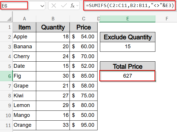
This version combines both conditions into a single line, summing all prices where quantity does not equal the value in E3.
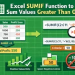
Sum Between Two Limits Using SUMIFS Function and Cell References
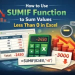
This method helps you calculate the total sum of values that fall between two numeric limits, which you define in cells. By using the SUMIFS function with greater than (>) and less than (<) conditions referencing these cells, you can dynamically control the range for summation.
We will find the total sum of prices where the quantities lie strictly between or inclusively between our specified lower and upper limits in different cells. This is useful for flexible filtering of data such as sales, scores, or quantities based on thresholds you can easily update.
Steps:
➤ In cell E5, enter the lower threshold value (for example, 15).
➤ In cell E7, enter the upper threshold value (for example, 30).
➤ Select a blank cell (e.g., E2) and enter this formula to sum values excluding the boundary values (strictly greater than lower threshold and less than upper threshold):
=SUMIFS(C2:C11, B2:B11, “>”&E5, B2:B11, “<“&E7)
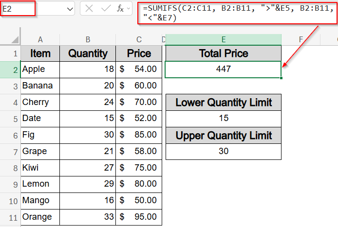
This formula will sum Price range where the Quantity is strictly greater than 15 and less than 30.
➤ Alternatively, to include the boundary values (sum prices where quantity is equal to or between 15 and 30), enter this formula in the same cell:
=SUMIFS(C2:C11, B2:B11, “>=”&E5, B2:B11, “<=”&E7)
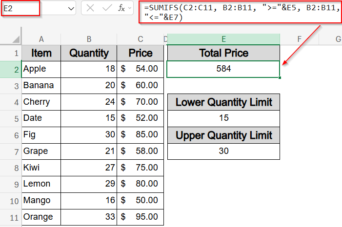
This will sum prices where the quantity is greater than or equal to 15 and less than or equal to 30.
Use SUMIF Function with Direct Constants Instead of Cell Values
This method lets you calculate the total sum of values between two fixed numeric limits by hardcoding those limits directly into the formula instead of using cell references. It’s useful when your threshold values don’t need to change often and you want a quick, straightforward calculation.
We will find the total sum of prices where the quantities are strictly greater than a lower limit and less than an upper limit, both written directly in the formula.
Steps:
➤ First, decide the numeric limits you want to use for your range. For example, a lower limit of 15 and an upper limit of 30.
➤ Next, select a blank cell where you want the sum result to appear, for example, E2.
➤ Now, enter the SUMIFS formula with the limits set as conditions like this:
=SUMIFS(C2:C11, B2:B11, “>15”, B2:B11, “<30”)
➤ This formula sums the values in the C2:C11 range where the corresponding quantities in B2:B11 are strictly greater than 15 and less than 30.
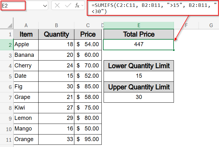
This will sum prices where quantity is greater than 15 but less than 30.
Subtract SUMIF Function to Calculate Closed Range Totals
This method calculates the total sum for values within a closed interval by subtracting two open-ended SUMIF calculations. Instead of directly summing between two limits, it sums all values above the lower limit and then subtracts the sum of values at or above the upper limit. This effectively gives the sum of values between the two thresholds.
We will find the total sum of prices where the quantity lies between the lower limit in E5 and the upper limit in E7, excluding the upper limit itself.
Steps:
➤ First, enter your lower threshold in cell E5 (for example, 16) and your upper threshold in E7 (for example, 33).
➤ Next, select a blank cell where you want the result, such as E2.
➤ Now, enter the formula that sums all prices with quantities greater than the lower limit, then subtracts the sum of prices where quantities are greater than or equal to the upper limit:
=SUMIF(B2:B11, “>”&E5, C2:C11) – SUMIF(B2:B11, “>=”&E7, C2:C11)
➤ Press Enter to calculate the total sum of prices where the quantity is strictly greater than the value in E5 and strictly less than the value in E7.
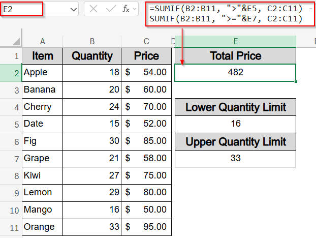
Now you have the total sum of prices where the quantity is strictly greater than the value in E5 and strictly less than the value in E7.
Use Dynamic Range with Named Table or Structured References to Find Total Sum
This method uses Excel Tables and structured references to create dynamic ranges that automatically adjust as your data grows or changes. Instead of regular cell ranges, you refer to table columns by name, which makes formulas easier to read and maintain.
We will find the total sum of prices where quantities fall between the lower limit in E5 and the upper limit in E7, using a named Excel Table called Table1.
Steps:
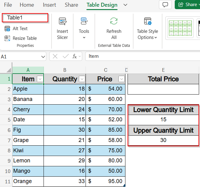
➤ First, convert your dataset into an Excel Table by selecting it and pressing Ctrl + T and it will automatically be named as Table1.
➤ Enter your lower threshold in cell E5 (e.g., 15) and your upper threshold in E7 (e.g., 30).
➤ Select a blank cell (e.g., E2) where you want the sum result to appear.
➤ Enter this formula using structured references to sum prices where quantities are greater than the lower limit and less than or equal to the upper limit:
=SUMIFS(Table1[Price], Table1[Quantity], “>”&E5, Table1[Quantity], “<=”&E7)
➤ Press Enter for output.
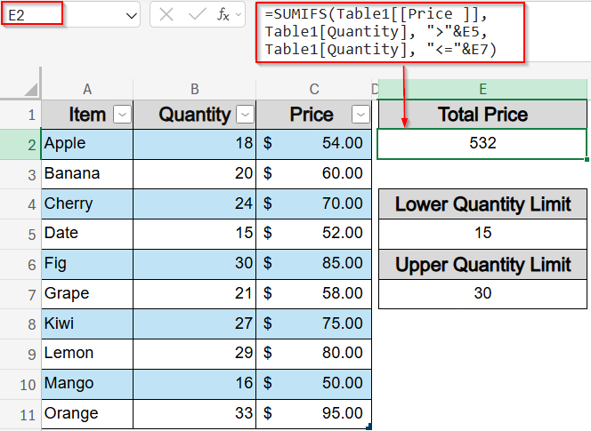
Now you have your total sum from a dynamic table which will automatically update as rows are added or removed from Table1.
Split SUMIF Function for Greater Than and Less Than a Cell Value
This method lets you calculate two separate totals, one for values greater than a specific number and another for values less than it. Instead of combining both conditions into one formula, you treat each range independently using two separate SUMIF functions.
We’ll sum quantities from column B based on whether the corresponding prices in column C are greater than or less than a given value. This technique is useful when you want to compare or display both sums side by side.
Steps:
➤ In E7, type the price limit you want to use (for example, 60).
➤ In E2, enter this formula to sum quantities where the price is greater than the value in E7:
=SUMIF(C2:C11, “>”&E7, B2:B11)
➤ Press Enter.
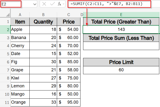
This calculates the total quantity where the price is greater than the limit in E7.
➤ In E4, enter this formula to sum quantities where the price is less than the value in E7:
=SUMIF(C2:C11, “<“&E7, B2:B11)
➤ Press Enter to view the results.
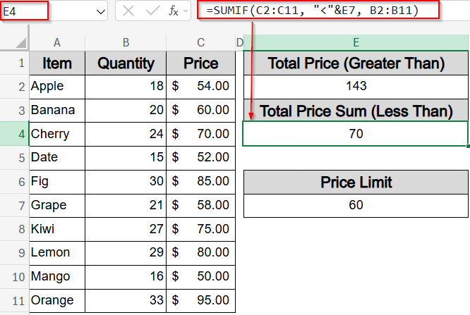
Now you have your total sum less than the Price Limit value.
Frequently Asked Questions
What does "sum if greater than and less than a cell value" mean in Excel?
It means adding up values from a dataset that fall strictly between two values stored in cells. The formula skips the exact boundaries and includes only the values greater than one cell and less than the other.
Can I include the boundary values in my sum?
Yes, you can include the boundary values by using greater than or equal to (>=) and less than or equal to (<=) in your formula. This way, the values matching the limits are also summed.
How do I exclude just one specific value from being summed?
To skip a single value, you can use two separate SUMIF functions: one for values below the target, and one for values above it. This approach completely ignores the specified number in your sum.
Is there a way to write the formula without using cell references?
Yes, instead of using separate cells for limits, you can directly enter the numbers into the formula. This is useful for static ranges where the limits won’t change and keeps the formula more compact.
Will these formulas update if I turn my data into a table?
Yes, when you use Excel Tables with structured references, your formulas automatically update. Any rows you add or delete are instantly reflected in the calculation, making your summaries more flexible and dynamic.
Wrapping Up
In this tutorial, we learned how to sum values in Excel based on whether they fall greater than and less than specific cell values. We covered multiple methods using functions like SUMIF, SUMIFS, subtraction methods, structured table references, and even how to exclude a single value completely. Each method serves a different scenario whether you want fixed ranges, dynamic cell-based limits, or flexible tables that grow with your data. Feel free to download the practice file and share your feedback.