The AVERAGEIF function in Excel is an effective tool for calculating the average of cells that meet a specific condition. In many real-world datasets, you often need to exclude zero values, ignore blanks, or focus on a subset of values that meet certain criteria such as only averaging positive sales, high quantities, or specific product categories. Whether you’re analyzing sales figures, tracking inventory, or reviewing performance data, this function allows you to calculate conditional averages that reflect only the data you care about.
In this article, we’ll learn how to use AVERAGEIF and AVERAGEIFS functions to exclude zeros, calculate averages between two values or dates, work with text-based conditions, and more with realistic examples and formulas that you can apply right away.
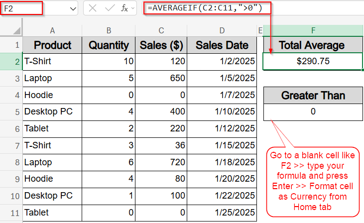
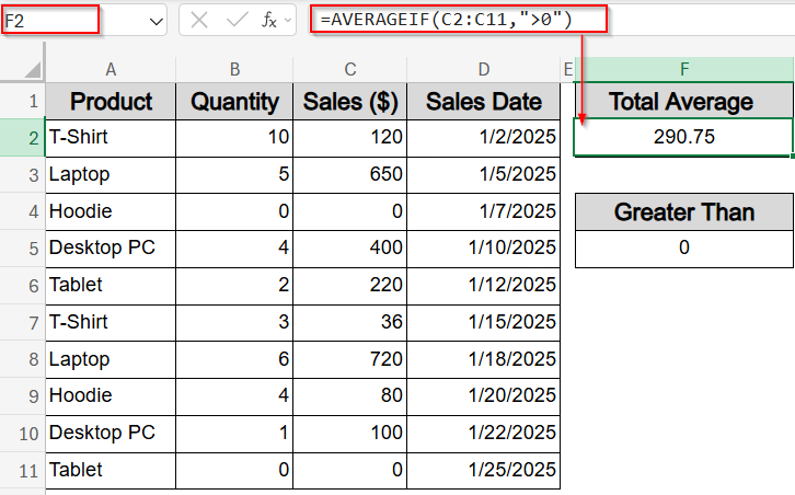
Steps to use AVERAGEIF greater than 0 in Excel:
➤ Click on a blank cell where you’d like the result to appear (e.g., F2).
➤ Enter the following formula:
=AVERAGEIF(C2:C11,”>0″)
Here, this formula tells Excel to average only the numbers in the Sales column (C2:C11) that are greater than zero.
➤ Press Enter to get the result.
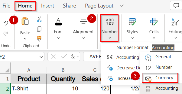
➤ Format the result as Currency or Number using the Home tab, if necessary.
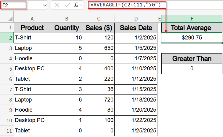
Determine Average for Values Greater Than Zero
In many sales datasets, you’ll encounter entries with zero values, often representing items that weren’t sold. Including these zeros can drag down your overall average. This method calculates the average of only those sales that are greater than zero. Our goal is to use the Sales column C to return the average of actual sales transactions, excluding rows where no sale occurred.
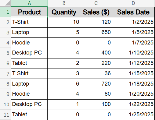
We will use a sample dataset containing products, their quantities sold, sale dates, and total sales amounts for demonstrating how AVERAGEIF function works with numbers, dates, and text conditions.
Steps:
➤ Click on a blank cell where you’d like the result to appear (e.g., F2).
➤ Enter the following formula:
=AVERAGEIF(C2:C11,”>0″)
Here, this formula tells Excel to average only the numbers in the Sales column (C2:C11) that are greater than zero.
➤ Press Enter to get the result.
➤ Format the result as Currency or Number using the Home tab, if necessary.
Now this gives the true average of positive sales, ignoring entries like returned items or non-purchases.
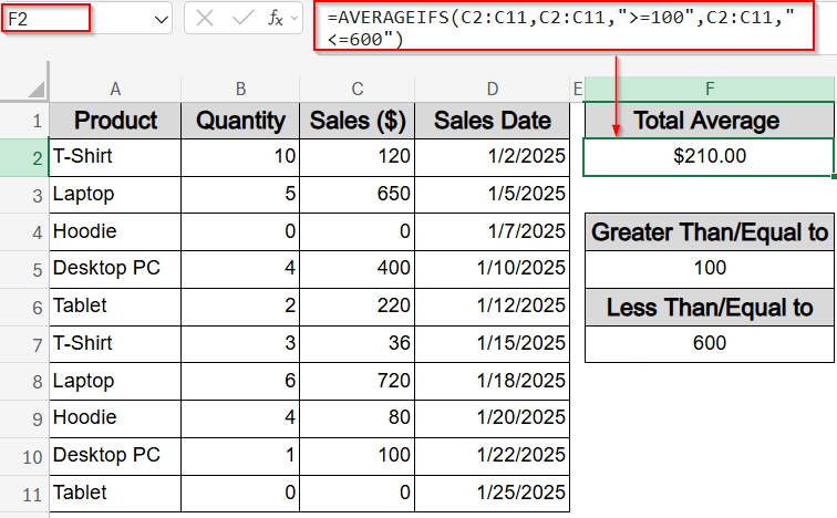
Find Average Within a Specific Numeric Range
This method is useful when you want to calculate the average for a defined sales range, for example, analyzing only mid-level transactions. Using the Sales column (C2:C11), we’ll calculate the average of all values that fall between 100 and 600. This helps you understand how mid-range sales are performing, without being skewed by very high or very low numbers.
Steps:
➤ Click on a blank cell where you want the result to appear, such as F2.
➤ Enter the formula:
=AVERAGEIFS(C2:C11,C2:C11,”>=100″,C2:C11,”<=600″)
➤ Press Enter to get the result.
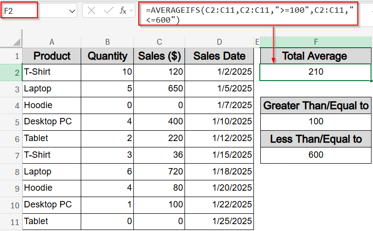
➤ Optionally, format the result as Currency or Number from the Home tab.

This formula tells Excel to average only the values in column C that are greater than or equal to 100 and less than or equal to 600. This provides a focused look at sales that fall within a typical operating range.
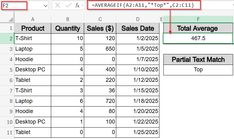
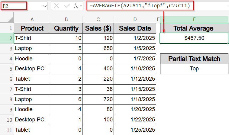
Calculate Average Based on Partial Text Criteria
This method helps you find the average sales for products whose names include specific text patterns. For example, using the Product column (A2:A11), we can average sales for any product containing the word “Top,” which would include items like “Laptop” or “Desktop PC“. This technique is useful when you want to group and analyze similar product categories without listing each name individually.
Steps:
➤ Select a blank cell where the result will appear, such as F2.
➤ Enter the formula:
=AVERAGEIF(A2:A11,”*Top*”,C2:C11)
➤ Press Enter to see the result.
➤ You can format the result as Currency or Number for clarity.

This formula works by averaging the values in the Sales column (C2:C11) only where the corresponding Product name contains the text “Top” anywhere in the string using wildcard * before and after “Top“.
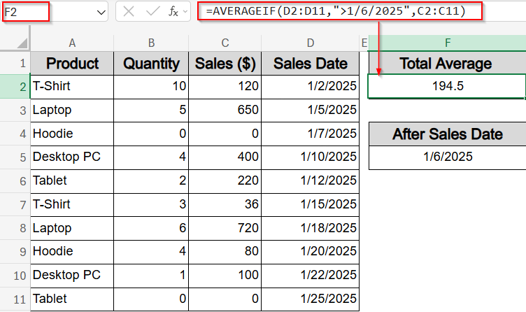
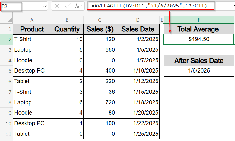
Evaluate Average for Dates after a Specific Day
This method allows you to find the average sales for all transactions that took place after a certain date, helping you analyze recent sales trends or performance. Using the Sales Date column (D2:D11), we can focus on data from a specific cutoff point onward such as January 6, 2025.
Steps:
➤ Select a blank cell to display the result, such as F2.
➤ Enter the formula:
=AVERAGEIF(D2:D11,”>1/6/2025″,C2:C11)
➤ Press Enter to calculate the average.
➤ Format the result as Currency or Number if needed.

This formula averages the sales amounts in column C where the corresponding sales date in column D is later than January 6, 2025, giving you insight into more recent sales performance.
Frequently Asked Questions
Can AVERAGEIF exclude zero values in calculations?
Yes, the AVERAGEIF function can exclude zeros by setting a condition like “>0”. This means only cells with values greater than zero are included in the average calculation, which is useful for ignoring zero sales or missing data points.
How is AVERAGEIFS different from AVERAGEIF?
While AVERAGEIF function handles a single condition, AVERAGEIFS function allows you to apply multiple conditions at once. This makes AVERAGEIFS function ideal for more complex scenarios where you need to filter data based on several criteria simultaneously.
Can I use wildcards with AVERAGEIF for partial text matches?
Yes. Using wildcards such as the asterisk (*) lets you include any cells where the text partially matches your criteria. This is helpful when product names or categories contain common keywords or patterns.
Is it possible to average values based on dates using AVERAGEIF?
Yes, AVERAGEIF function can use date criteria to average only those values where dates fall before or after a specific point. This is particularly useful for analyzing sales trends or performance within certain time frames.
Do I need to format the result after using AVERAGEIF or AVERAGEIFS?
It’s best to format the results for clarity. Applying Number, Currency, or Percentage formats ensures the output is easy to interpret and aligns with your dataset’s context which helps to present your analysis professionally.
Wrapping Up
In this tutorial, we explored how to use the AVERAGEIF and AVERAGEIFS functions in Excel to calculate averages based on various conditions. Whether you want to exclude zero values, focus on specific numeric ranges, filter by partial text matches, or analyze data after certain dates, these methods provide flexible ways to handle your sales data efficiently. Feel free to download the practice file and share your feedback.