A Pareto chart is an efficient visual tool that highlights the most significant factors in a dataset. It combines a bar graph showing individual values in descending order with a line graph displaying cumulative percentages. This dual-visual format makes it ideal for applying the 80/20 rule, helping you quickly identify which few categories are causing most of the impact whether it’s customer complaints, defects, or sales performance.
In this article, we’ll learn how to create a Pareto chart in modern Excel versions using its built-in features and apply manual techniques for older Excel versions. Let’s get started.
Steps to make a pareto chart in Excel:
➤ Select your data range, including headers (A1:B6).
➤ Go to the Insert tab.
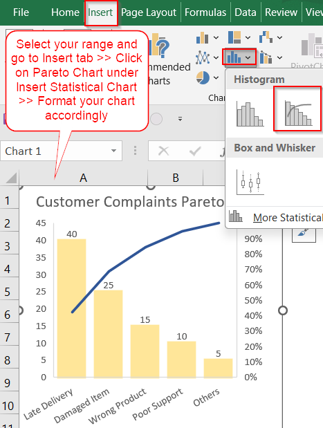
➤ Click Insert Statistic Chart >> Choose Pareto from the Histogram dropdown.
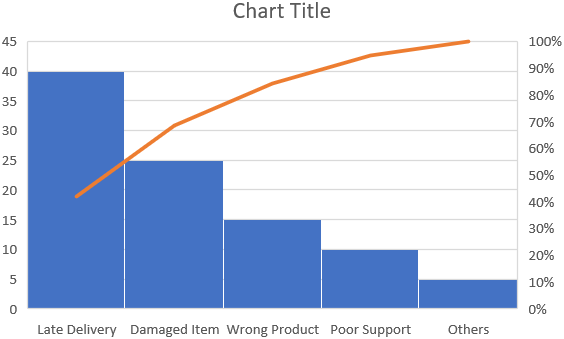
➤ Excel will instantly create a combo chart with bars sorted from largest to smallest and a line chart showing cumulative percentages.
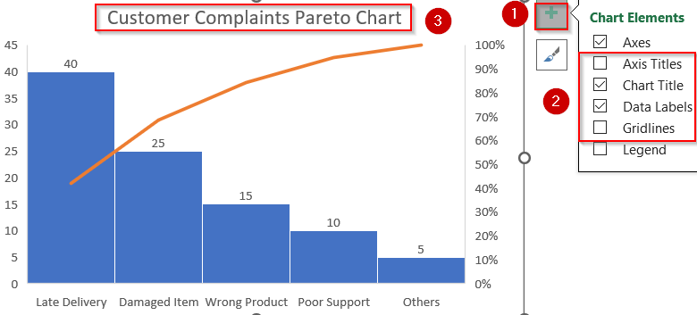
➤ Use Chart Elements (the plus icon) to add Data Labels or Axis Titles for clarity. Uncheck Gridlines if needed and edit Chart Title according to your preference.
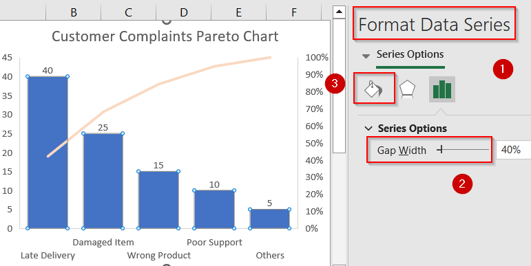
➤ To customize further, right-click on the bars and click on Format Data Series. Adjust Gap Width, Fill color, line styles, etc as preferred. You can also format your horizontal and vertical axes by clicking on them.
Create a Pareto Chart Using Excel’s Built-in Tool (Excel 2016+)
If you’re using Excel 2016 or later, the easiest way to visualize which categories have the greatest impact is by using the built-in Pareto chart feature. This tool creates a dual-axis chart with descending bars for frequency and a cumulative line that helps highlight the 80/20 relationship. The output will be a Pareto chart where bars represent complaint counts (from highest to lowest), and the line shows the cumulative percentage to help you identify the vital few issues that make up the bulk of complaints.
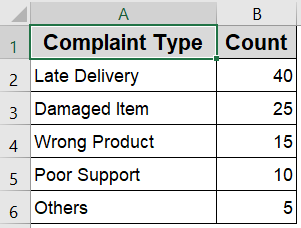
To demonstrate how a Pareto chart works, we’ll use a sample dataset showing different types of customer complaints and how frequently each one occurs. The goal is to identify which issues are most common so you can prioritize them effectively.
Steps:
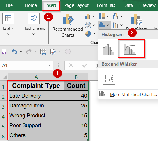
➤ Select your data range, including headers (A1:B6).
➤ Go to the Insert tab.
➤ Click Insert Statistic Chart >> Choose Pareto from the Histogram dropdown.
➤ Excel will instantly create a combo chart with bars sorted from largest to smallest and a line chart showing cumulative percentages.
➤ Use Chart Elements (the plus icon) to add Data Labels or Axis Titles for clarity. Uncheck Gridlines if needed and edit Chart Title according to your preference.
➤ To customize further, right-click on the bars and click on Format Data Series. Adjust Gap Width, Fill color, line styles, etc as preferred. You can also format your horizontal and vertical axes by clicking on them.
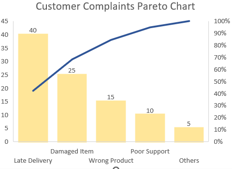
Now we have our customized Pareto chart that automatically calculates and plots the cumulative percentage, so we don’t need to calculate it manually.
Manually Create a Pareto Chart in Older Excel Versions
If you’re using Excel 2013 or earlier, you can create a Pareto chart manually by sorting your data and calculating cumulative percentages yourself. This method uses a combination of a column chart for counts and a line chart for the cumulative total, letting you visualize the most significant categories clearly without built-in tools. Let’s begin.
Steps:
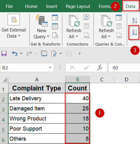
➤ Select range B2:B6 to sort the data in descending order by Count and click on the Largest to Smallest button from the Data tab.
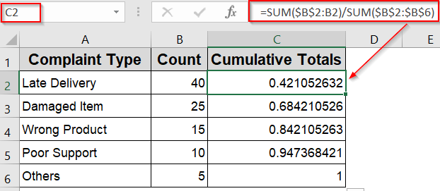
➤ Add a new column to calculate cumulative totals.
➤ Add another column to calculate cumulative percentage using this formula:
=SUM($B$2:B2)/SUM($B$2:$B$6)
➤ Click the bottom-right corner of that cell (the fill handle) and drag it down to apply the formula to the rest of the rows.
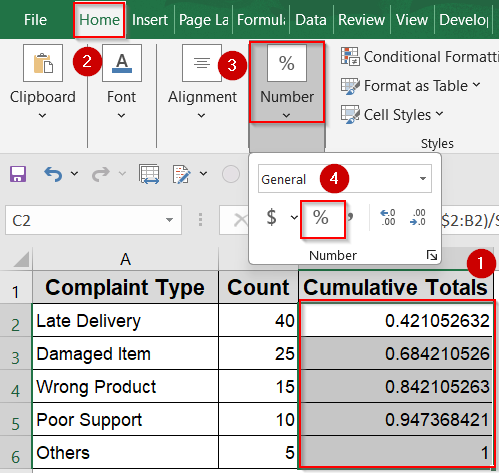
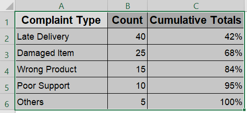
➤ Then format range C2:C6 as a percentage from the Home tab under Number group.
➤ Now select the entire range A1:C6 including headers.
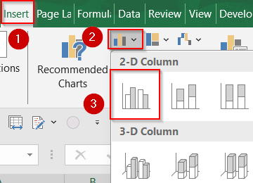
➤ Go to the Insert tab, and choose a 2-D Clustered Column chart.
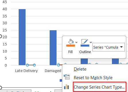
➤ On the chart, right-click the Cumulative Totals bars, choose Change Series Chart Type.
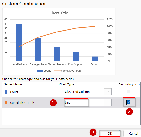
➤ Switch Cumulative Totals to a Line chart and check the box for Secondary Axis.
➤ Click OK to save changes.
➤ Finally, customise as needed using Chart Elements and Format Data Series.
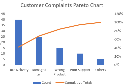
You’ll now have a functioning Pareto chart with bars for counts and a line for cumulative percentage, even in legacy Excel versions.
Frequently Asked Questions
What is a Pareto chart in Excel?
A Pareto chart combines a descending bar chart and a cumulative percentage line. It helps identify the most significant factors in your data, highlighting the vital few causes responsible for the majority of an effect.
Can I create a Pareto chart in all Excel versions?
Excel 2016 and later have a built-in Pareto chart feature. For older versions like Excel 2013 or earlier, you need to create one manually by sorting data and combining column and line charts with cumulative percentages.
How do I calculate the cumulative percentage for a Pareto chart?
Cumulative percentage is calculated by dividing the running total of values by the overall total sum. In Excel, use a formula like =SUM($B$2:B2)/SUM($B$2:$B$6) and format the result as a percentage.
Why won’t Excel create a Pareto chart automatically?
Excel requires data sorted in descending order and cumulative percentages for a Pareto chart. Built-in charts handle this automatically in newer versions, but manual steps are needed in older Excel versions for accurate results.
Can I customize colors in a Pareto chart?
Yes. Excel allows customization of bar colors, line styles, and markers. You can highlight important categories by changing colors or add data labels for clarity to make the chart more informative and visually appealing.
Wrapping Up
In this tutorial, you learned how to make a Pareto chart in Excel using both the built-in option for Excel 2016+ and a manual workaround for older versions. Whether you’re solving customer service issues or analyzing sales problems, a Pareto chart helps you focus on the most impactful factors fast. Choose the method that fits your Excel version and needs. Feel free to download the practice file and share your feedback.