IF Function in Google Sheets

The Google Sheets IF function is one of the most commonly used logical functions that helps you make decisions based on conditions. It allows you to create conditional logic in your spreadsheets performing one action if a condition is true and a different action if the condition is false. This function brings logic into your data so that the sheet can respond automatically based on the rules.

In this article, we will discuss a complete guide with formula examples about IF function in Google Sheets.

---

Syntax of IF Function in Google Sheets

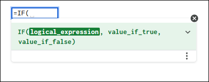
The syntax of the IF function defines how the formula is structured and which arguments it accepts. The function requires three arguments.

• logical_expression: This is the condition for testing (e.g., C2 > D2). It must result in either TRUE or FALSE.
• value_if_true: This is the action or value the formula returns if the logical_expression is TRUE.
• value_if_false: This is the action or value the formula returns if the logical_expression is FALSE.

---

Using IF Function to Check If Cell is Empty or Not Empty

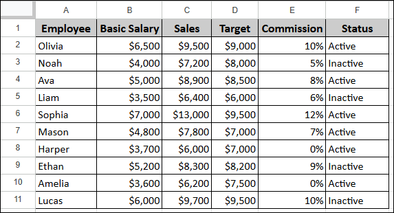
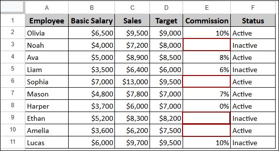
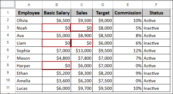
One of the most frequent uses of the IF function is to check if a cell is missing data (empty) or contains data (not empty). For our examples, we will use a sample sales dataset containing Employee, Basic Salary, Sales, Target, Commission and Status.

If Cell Is Empty

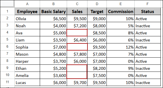
To avoid calculation errors caused by blank cells, you can use the built-in ISBLANK function within the IF function. In the sample data you will see some missing values in the Sales column (Column C).

Here, we will check if the Sales value (Column C) is missing. If it is, we will return the text “Sales Missing”; otherwise, we calculate the Bonus Amount (Sales * Commission).

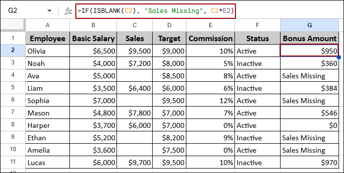
➤ Select cell G2, write down the formula below, press ENTER, and drag the Fill Handle down.

Formula Breakdown:

• ISBLANK(C2): Checks if cell C2 is empty (TRUE if blank, FALSE if not).
• “Sales Missing”: The result returned if C2 is blank (TRUE).
• C2*E2: The calculation performed if C2 is not blank (FALSE).

The output shows the calculated bonus amount for employees with sales data, and the text “Sales Missing” is displayed where the sales field (Column C) was blank.

If Cell Is Not Empty

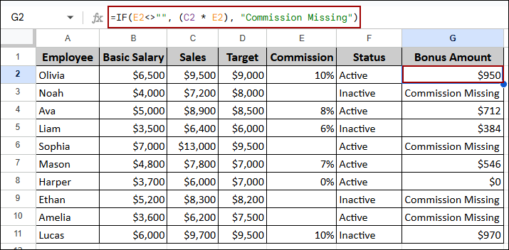
Alternatively, you can test if a cell is not empty by using the not equals operator (<>) along with the IF function. Suppose we have the same dataset with some blank cells in the commission column. We will use the IF function to calculate the Bonus Amount only if a Commission value (Column E) is present. If the commission is missing (empty), it will return “Commission Missing”.

➤ Choose a cell G2, write down the formula below, press ENTER and pull the Fill Handle down to fill.

Formula Breakdown:

• E2<>””: Checks if E2 is not equal to an empty string (“”).
• (C2 * E2): The calculation performed if E2 is not empty (TRUE).
• “Commission Missing”: The text returned if E2 is empty (FALSE).

This formula calculates the bonus amount only when the Commission cell (Column E) is filled. It returns “Commission Missing” where blank cells appear.

---

Handling Zero and Blank Cells with IF Function in Google Sheets

When dealing with financial or inventory data, you often need to distinguish between a cell that is truly blank (missing data) and a cell that contains a zero (valid data). In this part, we will discuss both scenarios using the IF function.

If Cell Is Blank Then Return Zero

When calculating total a blank cell must be treated as a zero to prevent a calculation error.

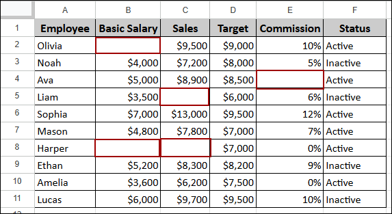
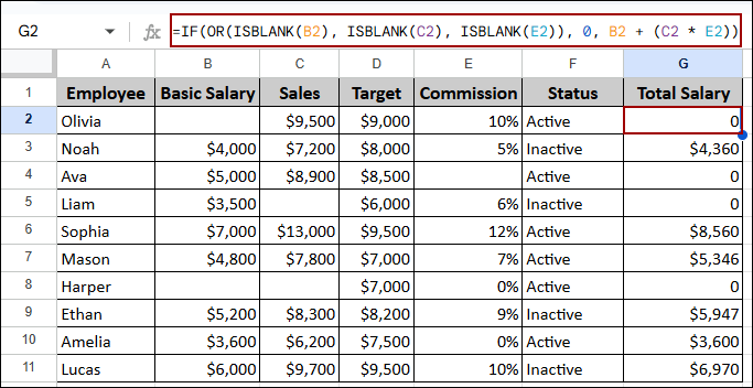
Suppose we have some blanks in different places for Basic Salary, Sales and Commission. We will use the OR function nested within IF to check if any required cell is blank, and return 0 in that case.

➤ Similarly, choose a cell G2, put the formula below, hit ENTER and drag down the Fill Handle.

Formula Breakdown:

• OR(ISBLANK(B2), ISBLANK(C2), ISBLANK(E2)): Returns TRUE if any of the three cells (B2, C2, or E2) are empty.
• 0: The value returned if any required cell is blank (TRUE).
• B2 + (C2 * E2): The Total Salary calculation performed if all cells contain data (FALSE).

As a result, we will get the output that records with missing values now correctly display a Total Salary of 0, instead of returning a calculation error.

If Zero Then Leave Blank

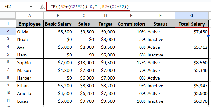
Sometimes, you might need to leave a cell blank if the result of a calculation is zero. Imagine we have some 0 values in the Basic Salary and Sales column. Here, using the IF function we will calculate the Total Salary but show a blank cell if the total is 0.

➤ Select cell G2, write down the formula below, hit ENTER and drag down the Fill Handle.

Formula Breakdown:

• (B2+(C2*E2))=0: Checks if the total calculated salary is exactly zero.
• “”: Returns an empty string (a blank cell) if the total is zero (TRUE).
• B2+(C2*E2): Returns the actual calculated total salary if it is not zero (FALSE).

The result successfully calculates the Total Salary but ensures that any employee whose total compensation is 0 displays a blank cell.

---

Applying IF Function to Check If Not and If Not Equal

You can combine the IF function with the NOT condition to invert a logical expression or the not equals operator (<>) to test if a specific value is present or not.

IF NOT

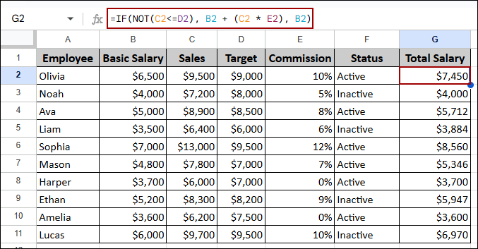
The NOT function inverts a true/false value. If the expression is TRUE, NOT make it FALSE, and vice-versa. Here, we will use the NOT function to calculate the Total Salary only if the Sales (C2) did not exceed the Target (D2). If sales did exceed the target, we will only pay the Basic Salary (B2) as a special case.

➤ Select cell G2, write down the formula below, press ENTER and fill the column by dragging the Fill Handle down.

Formula Breakdown:

• NOT(C2>D2): Returns TRUE only if C2 is not greater than D2.
• B2 + (C2 * E2): The full salary calculation returned if sales did not exceed the target (TRUE).
• B2: Only the basic salary returned if sales did exceed the target (FALSE).

The output applies the full calculation (Basic Salary + Bonus) only when the Sales did not reach the Target. If the Target was exceeded, the result is restricted to the Basic Salary alone.

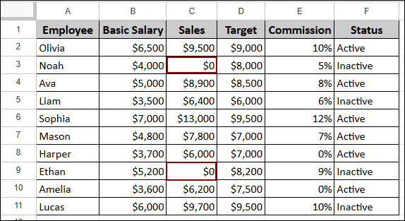
IF NOT Equal

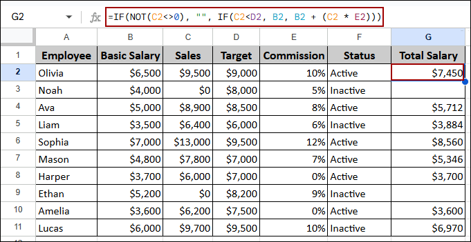
To check if a cell value is not equal to a blank cell and then perform a nested IF check, you can use the NOT function with equal operator. Suppose, we have some 0 sales for some employees in the dataset. Here, we will calculate the total salary only if the Sales (C2) cell is not blank . If C2 is not blank, we then check if C2 is less than D2, returning the Basic Salary (B2) or the Total Salary calculation.

➤ Choose a cell G2, type the formula below, click ENTER and drag down to fill.

Formula Breakdown:

• NOT(C2<>””): Checks if C2 is not equal to an empty string (i.e., checks if C2 is equal to an empty string).
• “”: Returns a blank cell if C2 is empty (TRUE for the outer IF).
• IF(C2<D2, B2, B2 + (C2 * E2)): The nested IF function is executed if C2 is not empty (FALSE for the outer IF), performing a final check for target achievement.

This way the final result ensures that if the Sales cell is blank, the output is blank. For all other entries, the salary is calculated, with some employees receiving only the Basic Salary due to the nested condition.

---

Google Sheets IF Function with AND and OR Conditions

For conditions that require testing multiple criteria simultaneously, you can nest the AND and OR functions within the logical_expression of the IF function. In this part, we will discuss both using the IF function with AND and OR conditions.

IF Function with AND

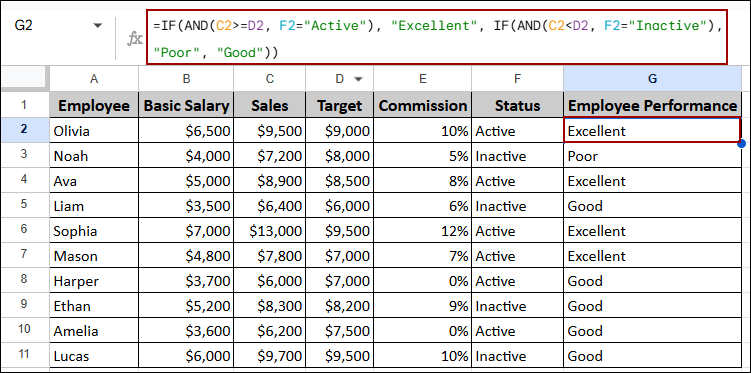
The AND function requires all conditions to be TRUE to return a TRUE result. Here, we will assign performance ratings based on two criteria: Sales (C) compared to Target (D) and Status (F).

➤ Select cell G2, put the formula below, press ENTER and drag down the Fill Handle.

Formula Breakdown:

• AND(C2>=D2, F2=”Active”): Checks if Sales meet Target AND Status is Active.
• “Excellent”: Returned if the first AND is TRUE.
• IF(AND(C2<D2, F2=”Inactive”), “Poor”, “Good” ): If the criteria for “Excellent” is not met, the formula proceeds to the nested IF to check other conditions.

Finally, we will get performance ratings to each employee based on the criteria defined by the AND conditions.

IF Function with OR

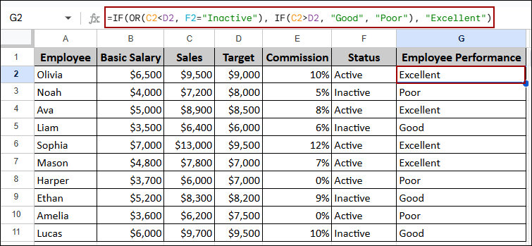
The OR function requires at least one condition to be TRUE to return a TRUE result. Here, we will use a simple logic to demonstrate the OR function: an employee is rated “Poor” if their Sales (C2) are less than their Target (D2) OR if their Status (F2) is “Inactive”.

➤ Choose a cell G2, type the formula below, click ENTER and drag the Fill Handle down.

Formula Breakdown:

• OR(C2<D2, F2=”Inactive”): Checks if Sales is less than Target OR if the Status is Inactive.
• IF(C2>D2, “Good”, “Poor”): If the OR test is TRUE (meaning a failure condition exists), the formula proceeds to the nested IF statement to refine the failure category.
• “Excellent”: Returned only if both conditions are FALSE (i.e., Sales > Target AND Status is Active).

The result provides a quick performance evaluation: employees are marked as “Poor” if they are inactive or missed their sales target, otherwise they are designated “Excellent”.

---

Using IF Function with Text

The IF function can perform powerful text-based filtering by checking for exact matches, partial matches, or matches within a list of possibilities. Suppose we have a dataset containing Product ID, Product Name, and Quality Check Report. Now, we will use the IF function to check for specific, partial and list of text.

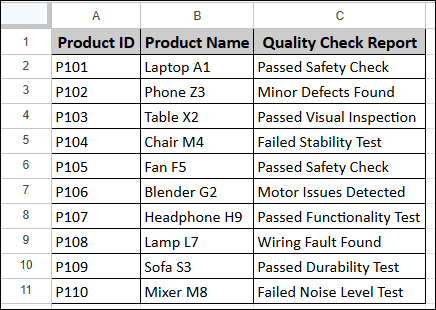
Cell Contains Specific Text

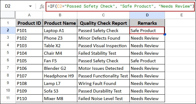
To check if a cell contains an exact string of specific text, we will use the standard comparison operators. Using the data of Quality Check Reports (Column C) , we want to mark a product as “Safe Product” only if the report is exactly “Passed Safety Check”. It means we’re returning values in another column based on text criteria.

➤ Select cell D2, write down the formula below, click ENTER and pull the Fill Handle down.

Formula Breakdown:

• C2=”Passed Safety Check”: Checks for an exact match of the text string.
• “Safe Product”: Returned if the text is an exact match (TRUE).
• “Needs Review”: Returned if the text is anything else (FALSE).

As a result, we will get the remarks with the exact text match “Passed Safety Check” labeled “Safe Product”, while all others as “Needs Review”.

Cell Contains Partial Text

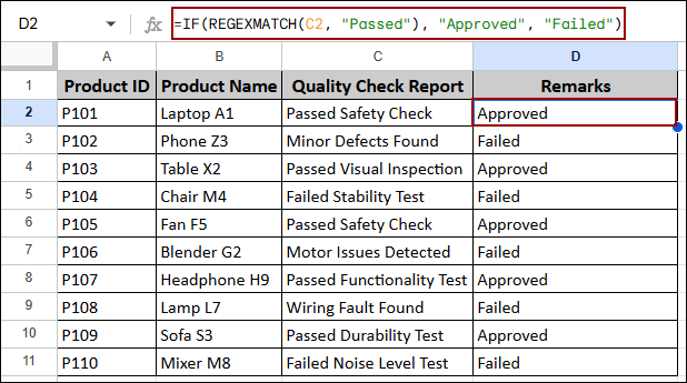
To check for a specific substring (part of the text) within a cell, we will combine IF with the REGEXMATCH function. Here, we will search for a text like “Passed” in the Quality Check Report.

➤ Select cell D2, write down the formula below, press ENTER and pull the Fill Handle down.

Formula Breakdown:

• REGEXMATCH(C2, “Passed”): Returns TRUE if the text “Passed” is found anywhere within the string in C2.
• “Approved”: Returned if the partial text is found (TRUE).
• “Failed”: Returned if the partial text is not found (FALSE).

The result simplifies the quality report into a clear pass/fail status: any report containing the word “Passed” is marked “Approved”, otherwise “Failed”.

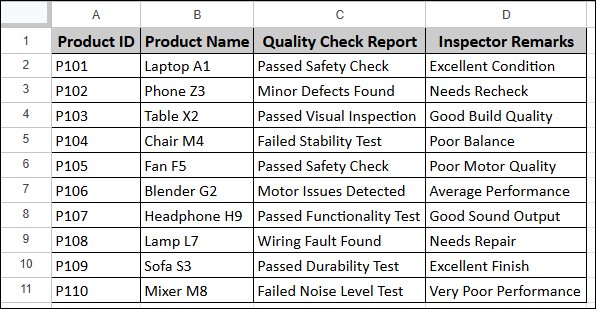
Cell Contains Text from List

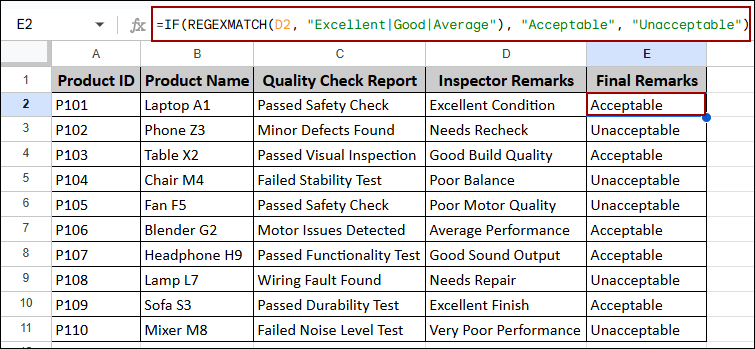
You can also check for multiple possible keywords simultaneously combining the IF and REGEXMATCH functions. Suppose we have the Inspector Remarks for the same dataset. Here, based on the Inspector Remarks (Column D) , we will mark a product as “Acceptable” if the remarks contain “Excellent”, “Good”, or “Average” .

➤ Select cell E2, type the formula below, click ENTER and pull the Fill Handle down.

Formula Breakdown:

• REGEXMATCH(D2, “Excellent|Good|Average”): Checks if D2 contains any of the three words separated by the OR symbol (|).
• “Acceptable”: Returned if any of the three keywords are found (TRUE).
• “Unacceptable”: Returned if none of the keywords are found (FALSE).

The output provides a final remarks for products with positive remarks like “Excellent”, “Good”, or “Average” are deemed “Acceptable”, consolidating several text inputs into one clear status.

---

Google Sheets IF Function with Multiple Conditions

While the combination of IF with AND and OR handles many scenarios, you can use nested IF or the dedicated IFS function for more complex data or multiple conditions.

Nested IF Function

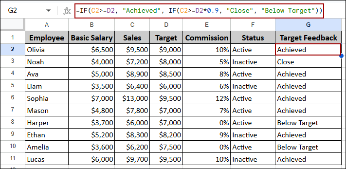
A nested IF function places one IF function inside another’s value_if_true or value_if_false arguments. This allows you to check a sequence of conditions. Here, we provide Target Feedback based on three levels. For Achieved: Sales (C2) > Target (D2), for Close: Sales (C2) > 90% of Target (D2*0.9) and for Below Target anything outside the conditions.

➤ Choose a cell G2, type the formula below, hit ENTER and drag down the Fill Handle.

Formula Breakdown:

• Outer IF: Checks for the “Achieved” condition first.
• Inner IF: If not Achieved (FALSE), the second IF checks for the “Close” condition.
• “Below Target”: If the second condition is also FALSE, the default value is returned.

Thus, the output successfully categorizes each employee’s sales performance into one of three distinct labels: Achieved, Close, or Below Target, based on the set of conditions.

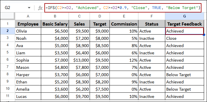
IFS Function

The IFS function is more efficient than nested IF, introduced specifically for checking multiple conditions. We will use the same three-level logic as above: C2>=D2, “Achieved”, C2>=D2*0.9, “Close”, TRUE, “Below Target” (The TRUE condition acts as the final ‘catch-all’ condition).

➤ Select cell G2, write down the formula below, click ENTER and pull the Fill Handle down.

As a result, we will get the same Achieved, Close, or Below Target labels using the IFS function.

---

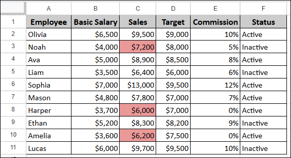
Using Google App Script to Check Cell Color

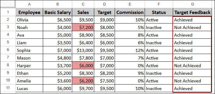
The standard IF function cannot check a cell’s formatting, such as its background color. To perform conditional logic based on cell color, you must use Google Apps Script. Suppose we have a sheet where sales below target are conditionally formatted (e.g., colored red).

To get the output we will create a new column naming Target Feedback.

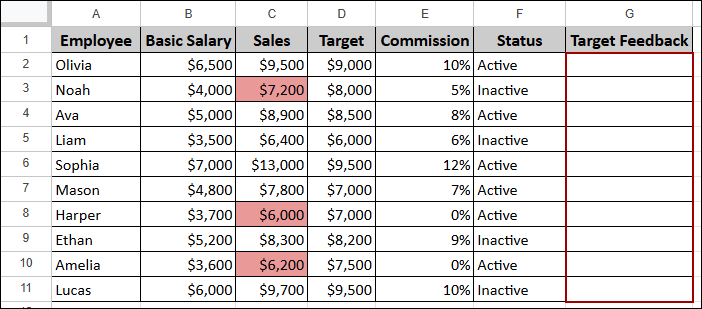
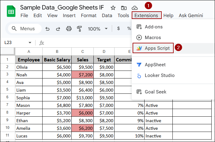
➤ Click Extensions in the menu and select Apps Script.

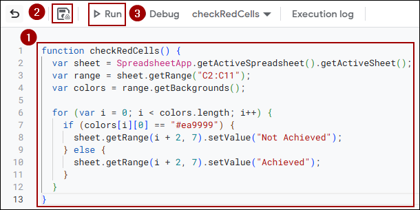
➤ In the script editor, paste the following code, save and run it.

function checkRedCells() {
var sheet = SpreadsheetApp.getActiveSpreadsheet().getActiveSheet();
var range = sheet.getRange("C2:C11");
var colors = range.getBackgrounds();
for (var i = 0; i < colors.length; i++) {
if (colors[i][0] == "#ea9999") {
sheet.getRange(i + 2, 7).setValue("Not Achieved");
} else {
sheet.getRange(i + 2, 7).setValue("Achieved");
}
}
}

Thus, the script marks the red backgrounded cells as “Not Achieved” and others as “Achieved”.

---

Frequently Asked Questions

Why does my IF formula return an error when checking a date?

Google Sheets stores dates as serial numbers. So, when you check dates in an IF statement, you should use the date’s serial number (e.g., DATE(2025, 1, 15)) or ensure the format matches the sheet’s default date format for a direct comparison.

Can IF evaluate background color or formatting?

No, the basic IF function works on cell values and logical expressions, not on cell formatting such as background color. For color‐based logic you need to use custom scripting or add‐ons.

Does the IF function care about the case of text (upper‐case vs lower‐case)?

No, text comparisons in IF are not case‐sensitive. For example, “apple” and “Apple” are treated as equal in this context.

---

Concluding Words

Above, we have covered a completed guide about IF function in Google Sheets. By combining its simple syntax with logical functions like AND, OR, and NOT, you can get your desired output with multiple conditions. Whether you are checking for missing data, assigning performance grades, or filtering text, the IF function provides the essential conditional logic to solve your problems. If you have any queries, feel free to share them in the comment section below.