
Extracting data based on a drop-down list selection in Excel allows you to make your worksheets interactive and easier to analyze. Instead of manually filtering rows every time, you can simply choose an option from a drop-down list, and Excel will automatically display only the data that matches your selection.
In this article, you’ll learn how to extract data based on a drop-down list selection in Excel using different methods suitable for both modern and older Excel versions.
Here’s how to extract data based on a drop-down list selection in Excel:
➤ Open your dataset in Excel with headers such as Region, Salesperson, Product, Quantity, and Revenue.
➤ Create a list of unique regions in a helper column or generate them automatically using =UNIQUE(A2:A11).
➤ Select a cell for the drop-down, go to Data tab >> Data Validation, choose List, and set the Source to the range with region names.
➤ Build an output table with the same headers as your dataset.
➤ Use the FILTER function to extract rows that match the drop-down selection. Type the following formula:
=FILTER(A2:E11, A2:A11=C14, “No data found”)
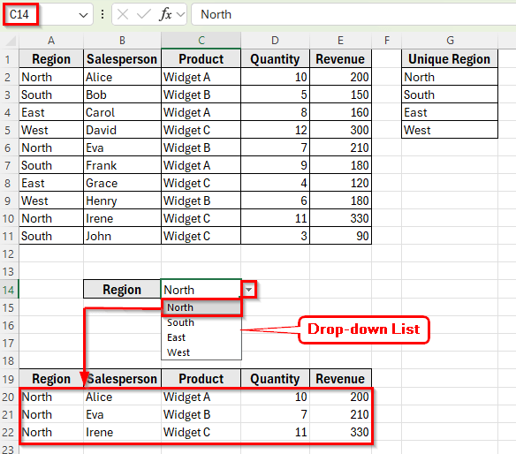
➤ Press Enter. Excel will now display all rows where the region matches the selected value in the drop-down cell. For example, if you select North, you’ll see only the sales records for Alice, Eva, and Irene.
Using the FILTER Function to Extract Data Based on Drop-Down Selection
In the following dataset, we have regional sales data. Column A lists the Region, Column B shows the Salesperson, Column C contains the Product, Column D records the Quantity Sold, and Column E displays the Revenue. Column F is empty, where we’ll display the extracted results based on the selected region.
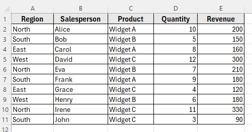
We’ll use this dataset to demonstrate different ways to extract data dynamically based on a drop-down list selection in Excel.
The FILTER function is the simplest and most efficient way to extract data based on a drop-down list in Excel. It automatically returns only the rows that meet the selected criteria and updates the results instantly when you change the drop-down selection. This function works in Excel 365 and Excel 2021.
Here’s how to do it:
➤ Open your dataset in Excel. Make sure your data has headers such as Region, Salesperson, Product, Quantity, and Revenue.
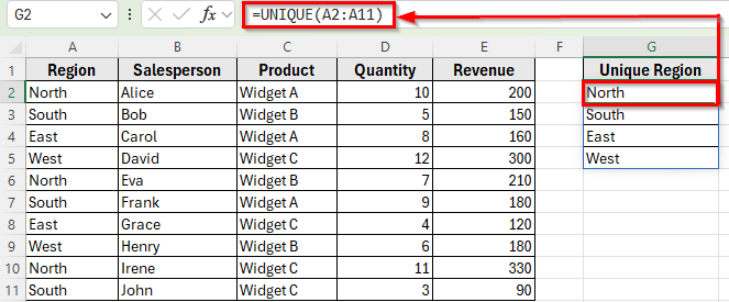
➤ In another column, for example column G, type or extract unique region names (North, South, East, West). You can also use the formula below to generate them automatically:
=UNIQUE(A2:A11)
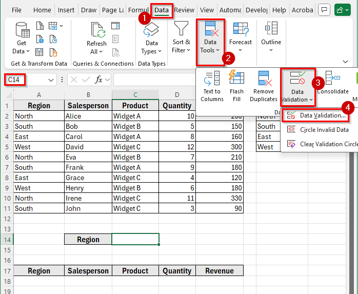
➤ Click on an empty cell, for example, C14, where you want the drop-down.
➤ Go to the Data tab >> Data Validation.
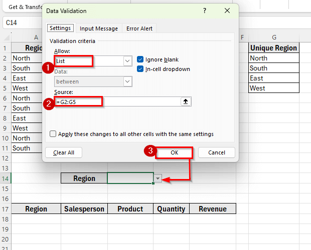
➤ In the Data Validation window, select List in Allow field.
➤ In the Source box, enter the range containing the region names, for example: =G2:G5.
➤ Click Ok. Now a drop-down list is created in cell C14
➤ Now, in another area such as starting from cell A17, create headers that match your dataset (Region, Salesperson, Product, Quantity, Revenue).
➤ Click on cell A18, under the first header, type the following formula:
=FILTER(A2:E11, A2:A11=C14, "No data found")
➤ Press Enter. Excel will initially display No Data Found because the drop-down cell is empty. When you select a region from the drop-down list, Excel will display all rows where the Region matches the selected value.
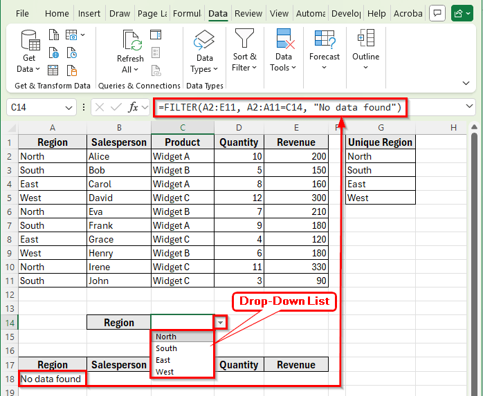
➤ Next, select a region, for example North, you’ll see only the sales records for Alice, Eva, and Irene.
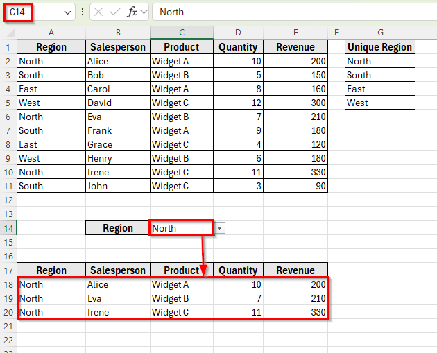
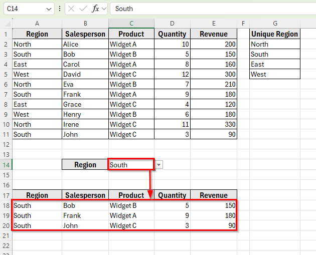
➤ Change the drop-down selection to test it. Try choosing another region such as South or West, and watch the extracted data update instantly.
Extract Data Based on a Drop-Down Selection for Multiple Criteria
Sometimes, you may want to extract data based on more than one condition. For example, filtering results not only by Region but also by Product.
Here’s how to do it:
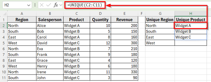
➤ In column H add a new list of Unique Products. Type this following formula in cell H2:
=UNIQUE(A2:A11)
➤ Press Enter. This formula extracts unique Product names such as Widget A, Widget B, Widget C.
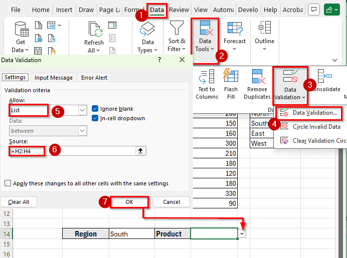
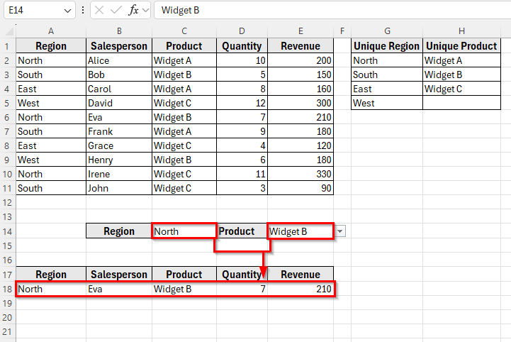
➤ Add another drop-down list for Product in cell E14, using the same Data Validation steps.
➤ Go to the Data tab and click Data Tools >> Data Validation.
➤ In the Data Validation window, select List in Allow field.
➤ In the Source box, type the Unique Product range, for example =H2:H4.
➤ Click Ok. Now a drop-down list is created in cell E14.
➤ Now, use the following formula in cell A18 to extract the results that match both Region and Product:
=FILTER(A2:E11, (A2:A11=C14)*(C2:C11=E14), "No match found")
➤ Press Enter. Excel will instantly display only those rows where both the selected Region and Product match.
➤ For example, if Region = North and Product = Widget B, Excel will display only the rows that match both conditions.
Using Helper Columns with INDEX and SMALL Functions
If you’re using an older version of Excel that doesn’t support the FILTER function, you can still extract data based on a drop-down selection by using helper columns along with the INDEX, IF, and SMALL functions. This method takes a few extra steps but works in all Excel versions.
Here’s how to do it:
➤ Open your dataset in Excel. Make sure your dataset contains the columns Region, Salesperson, Product, Quantity, and Revenue. Suppose your data range is A2:E11.
➤ Select cell C14, go to the Data tab then click Data Validation.
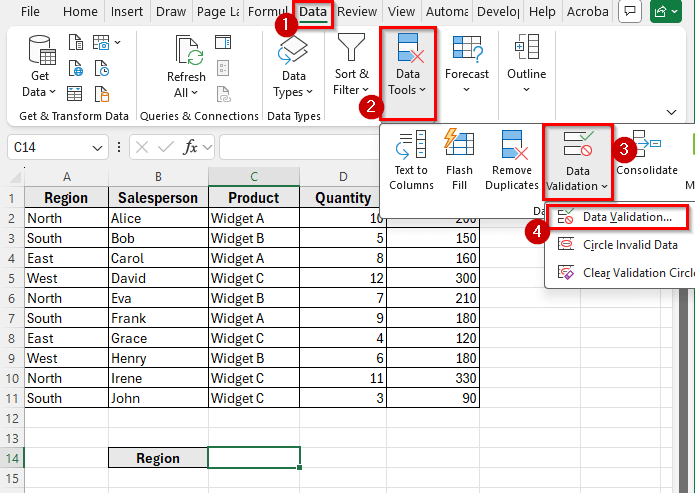
➤ In the Data Validation window, select List in Allow field and in Source box type =A2:A11 or a unique list if you prefer.
➤ Click Ok.
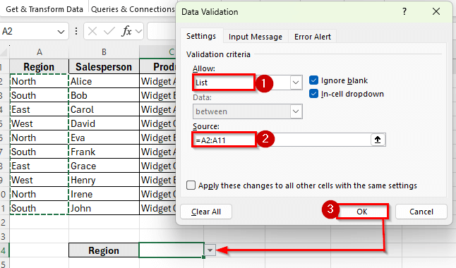
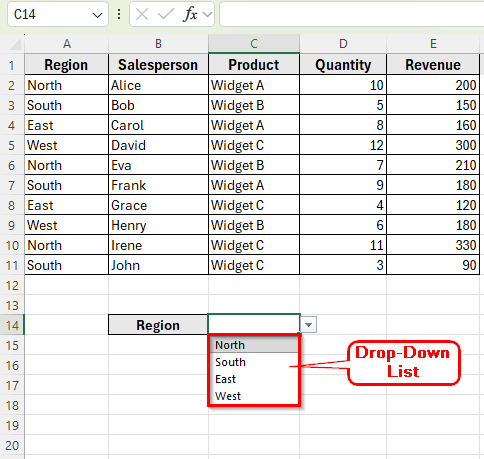
➤ Now C14 is the region selector such as North, South, East, West.
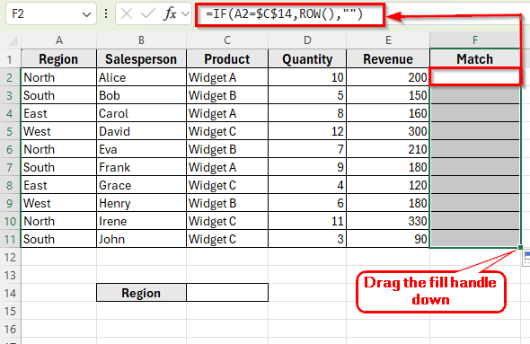
➤ Insert a helper column to mark matching rows. In column F, create a new header called Match.
➤ In cell F2, enter the following formula:
=IF(A2=$C$14,ROW(),"")
➤ Press Enter and drag the fill handle down to copy the formula for the rest of the rows.
➤ Here, $C$14 refers to the drop-down cell where you select the region. This formula will return the row number if the region matches the selected value and leave the cell blank otherwise.
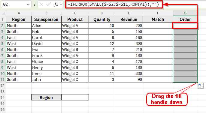
➤ Create another helper column to list matching row numbers in order. In column G, add a new header called Order.
➤ In cell G2, enter the following formula:
=IFERROR(SMALL($F$2:$F$11,ROW(A1)),"")
➤ Press Enter and drag the fill handle down to copy the formula for the rest of the rows.
➤ This formula lists all row numbers where the condition in column F is true, one by one.
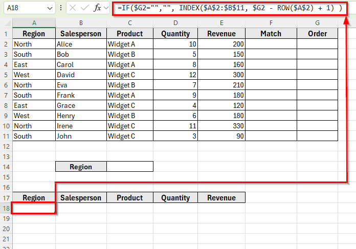
➤ Now, in another area such as starting from cell A17, create headers that match your dataset (Region, Salesperson, Product, Quantity, Revenue).
➤ Under the first header in cell A18, enter the following formula:
=IF($G2="","", INDEX($A$2:$A$11, $G2 - ROW($A$2) + 1) )
➤ Press Enter. Drag the fill handle down to cell A27 to copy the formula for the rest of the rows.
➤ Next, copy this formula across to the next columns for Salesperson, Product, Quantity, and Revenue, updating the column references accordingly:
For Salesperson type this formula in cell B18:
=IF($G2="","",INDEX($B$2:$B$11,$G2-ROW($A$2)+1))
For Product type this formula in cell C18:
=IF($G2="","",INDEX($C$2:$C$11,$G2-ROW($A$2)+1))
For Quantity type this formula in cell D18:
=IF($G2="","",INDEX($D$2:$D$11,$G2-ROW($A$2)+1))
For Revenue type this formula in cell E18:
=IF($G2="","",INDEX($E$2:$E$11,$G2-ROW($A$2)+1))
➤ Press Enter after applying each formula, then drag the fill handle down to row 27 in every column to extract all matching records.
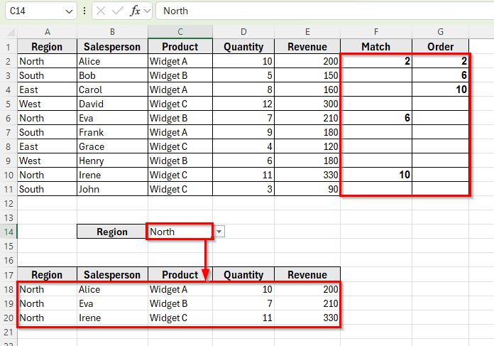
➤ Now, select a region from the drop down list, you’ll see the extracted dataset instantly update based on your selection.
➤ The formulas in the helper column dynamically identify the matching rows for the selected region, and the INDEX formula in the extracted table retrieves the related records for each column.
Downloadable Resources
Get our practice workbook or necessary files that we have worked with to prepare this article.
Extract Data Based on Dropdown List Selection.xlsx
Frequently Asked Questions
How do I extract data in Excel based on a single drop-down list?
Select the cell where you want the drop-down. Go to Data >> Data Validation, select List under Allow. In the Source box, enter the range containing your options. After creating the list, apply a FILTER or INDEX formula to display only the rows that match the selected value.
Why does my drop-down return blank or no data?
Blanks appear when there’s no match between the selected value and your dataset. Make sure your drop-down items exactly match the entries in your data columns. Also, avoid extra spaces or inconsistent spellings.
Can I make the extracted table update automatically?
Yes. Both FILTER and INDEX methods update results instantly when a new value is selected in the drop-down list. You can also convert your dataset into an Excel Table to ensure new rows are included automatically.
Wrapping Up
Extracting data based on a drop-down list selection in Excel makes your spreadsheets more dynamic and user-friendly. It allows you to control which records appear by simply selecting a value, saving time on manual filtering.
You can use the FILTER function for instant results while using Excel 365. Older versions of Excel don’t support this function, so you can apply helper columns with INDEX and SMALL instead.
This technique works perfectly for building interactive dashboards, sales summaries, and performance reports that update automatically based on user selections and changing data.