For better navigation in a complex workbook, Excel allows you to create dynamic hyperlinks that link to another sheet based on a cell value. Dynamic hyperlinks change their destination automatically based on the value in a cell.
For this, we can use the hyperlink option from the context menu or the HYPERLINK function. You can also combine additional functions, such as MATCH and INDEX, for lookup and conditional hyperlinks.
Steps to create a hyperlink using the context menu:
➤ Select the cell where you want to create the hyperlink and right-click on it. From the Context menu, choose Link/Hyperlink.
➤ As the Insert Hyperlink dialog box opens, click on Place in This Document from the Link To group.
➤ In the Type the Cell Reference box, enter the cell reference based on whose value you want to create the hyperlink. Click on the sheet name containing the cell reference from the given options in the next box. Press Ok to create the hyperlink.

This article covers all other methods of hyperlinking based on a value in a different sheet, including the use of the Drag & Drop technique and functions such as HYPERLINK, INDEX, and MATCH.
Create a Hyperlink Using the Drag and Drop Technique
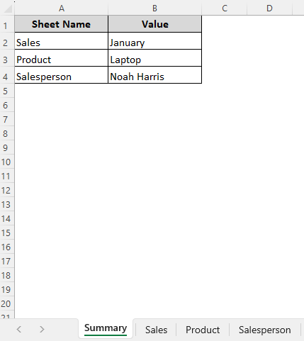
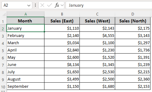
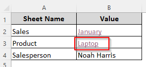
In our sample dataset, we have a summary sheet with a few sheet names in Column A. The values based on which we’ll link the sheets are in Column B. We’ve picked one value from each sheet (Sales, Product, and Salesperson). For easy demonstration, we’ll use a different method for each sheet and value.
While this is the quickest method to link two sheets based on value, it requires precise control over your device. For this method, we’ll hyperlink the cell from the Sales sheet that contains the value January. Here’s how to create a hyperlink in the Summary sheet by dragging a cell and dropping it in the destination sheet.
➤ As this method doesn’t work for unsaved workbooks, press Ctrl + S to save your Excel file.
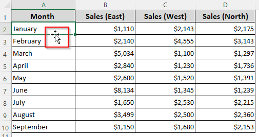
➤ Select the cell containing the reference cell value from the destination sheet (Sales). Hover the pointer on the cell’s border, right-click, and hold the four-sided arrow sign.
➤ As you hold the button, press the Alt key on your keyboard and hold it too. Now, use your touchpad to drag the right mouse button to the bottom of the screen where the sheet names are. Hover over the sheet where you want the hyperlink (Summary).
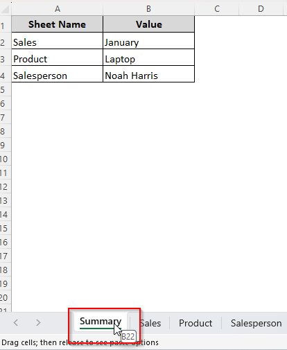
➤ Once the Summary sheet is activated, release the Alt key, but hold the mouse button.
➤ Use the touchpad again to drag the mouse pointer and place it over the cell where you want the link (B2). Now, release your mouse button and Excel will open a pop-up menu.
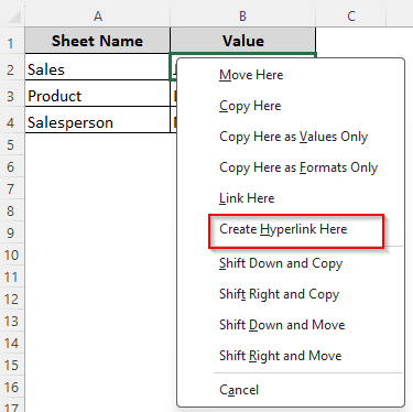
➤ Select Create Hyperlink Here and the two sheets are now linked.
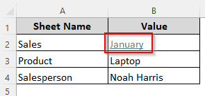
➤ When you click on the hyperlink, it will take you to the specific cell of the destination sheet containing the value you want to see. Here, the link takes us to the Sales sheet cell containing the value January.
Add a Hyperlink to a Cell Using the Context Menu Option
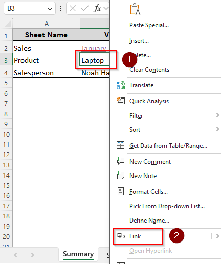
Excel’s Context menu has a direct option to create a hyperlink and decide where to place the link and which cell you’re referencing. We’ll link a cell from the Product sheet containing the value Laptop. Below are the steps:
➤ Right-click on the cell where you want the hyperlink (B3). Select Link (or Hyperlink) from the Context menu.
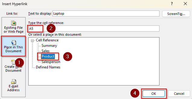
➤ When the Insert Hyperlink dialog box appears, select Place in This Document in the Link To group on the left.
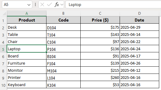
➤ Go to the Type the Cell Reference box and type the cell reference based on whose value you want to create the hyperlink. We entered A5 for the value Laptop in the Product sheet.
➤ Proceed to the Select a Place in This Document group. In the Cell Reference group, click on the destination sheet name (Product). Finally, click Ok.
➤ Excel adds a hyperlink to your selected cell.
➤ Here’s where our hyperlink takes us:
Use the HYPERLINK Function to Link Sheets Based on Cell Value
In the two arguments for the HYPERLINK function, you need to enter the link location and a friendly name (optional) that appears as the linked text. With this function, we’ll link the cell from the Salesperson sheet containing the name Noah Harris. Let’s get to the steps:
➤ Select the cell where you want to place the link and make sure it’s empty. If the cell already contains a value, copy it to a different location, and we can use it in the formula as the display text.
➤ In the empty cell, insert the following formula and press Enter.
=HYPERLINK("#'Salesperson'!A3", "Noah Harris")
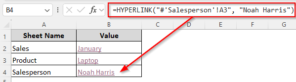
➤ Here, the # tells Excel the link is within the same workbook. ‘Salesperson’!A3 refers to the destination cell (A3 in the Salesperson sheet). Finally, “Noah Harris” is the display text for the link.
➤ Replace the display text, destination cell, and sheet name according to your dataset.
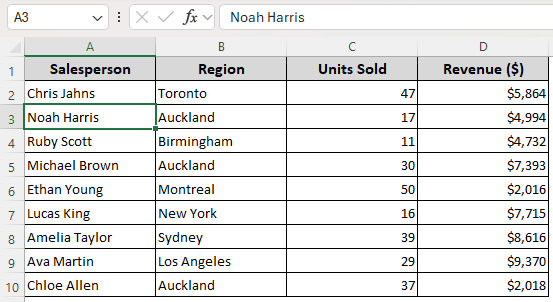
➤ Here’s the linked sheet:
Create Hyperlink with Dynamic Values
With this method, we can make our lookup cell values dynamic. So, every time you change the cell value, the link will update and redirect to another sheet’s cell where the value is found.
In our current sheet (Dynamic Values), we have created a drop-down list with a few values from the Product sheet in cell A2.
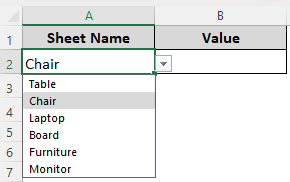
In cell B2, we’ll create a dynamic hyperlink that directs us to the correct cell containing the product name in cell A2. Let’s get to the steps:
➤ Select cell B2 to create the hyperlink and enter the following formula:
=HYPERLINK("#"&CELL("address",INDEX(Product!A2:A10, MATCH(A2,Product!A2:A10,0))),"Find in Workbook")
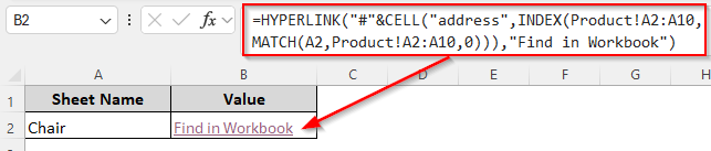
➤ Here, Product is the name of the destination sheet, A2:A10 contains the lookup values in the destination sheet, A2 is the cell containing the lookup value in the current sheet (Dynamic Values), and Find in Workbook is the display text. Replace the values as needed.
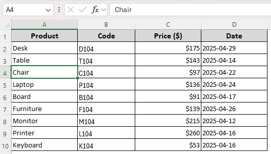
➤ When we choose Chair from the drop-down, here’s the output:
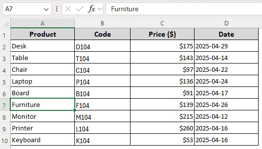
➤ As we change the value, the formula gives a different result:
Create Hyperlink with Dynamic Values and Sheet References
While the previous method deals with dynamic values, here we’ll make the sheet reference dynamic too. Our current sheet (Dynamic Values & Sheets) has 3 tab names in Column A (Sales, Product, and Salesperson) and 3 cell references in Column B (A4, B5, and C10).
If needed, you can create a drop-down with the values. This method creates a hyperlink based on the two lookup values in the same row. Here are the details:
➤ In an empty cell (C2) where you want the first hyperlink, insert this formula and press Enter:
=HYPERLINK("#'" & A2 & "'!" & B2, "Find in Workbook" & A2 & " " & B2)
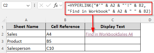
➤ Here, A2 contains the destination sheet name (Sales) and B2 contains the destination cell reference (A4). Change the cell references to match your data source.
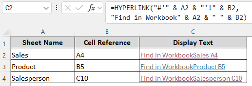
➤ After pressing Enter, you can drag the formula down to create hyperlinks for the remaining cells.
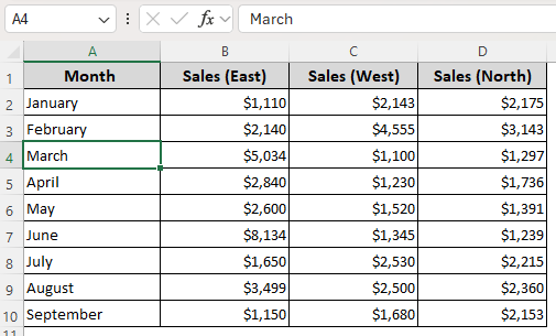
➤ Here’s what happens when we click on the first link:
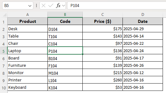
➤ Check out the result for the second link:
Frequently Asked Questions
How to hyperlink based on a range in another sheet?
To create a hyperlink that jumps directly to a specific range (not just one cell) in another sheet, use the HYPERLINK function and specify the range address. We want a link that takes us to the Sales sheet range A1:A10. So, we entered:
=HYPERLINK("#'Sales'!A1:A10", "Go to Sales Data")
When we click on the hyperlink text Go to Sales Data, Excel takes us to the Sales sheet, with A1:A10 selected (the top-left cell of that range becomes active).
How do you link to another workbook based on a cell value in Excel?
First, place the workbooks in the same folder on your device. To create a hyperlink to cell A5 of the Revenue sheet of AccountsBook2, enter this formula in your current workbook:
=HYPERLINK("[AccountsBook2]Revenue!C5","Follow Link")
Replace the values to match your source data.
How do you edit a hyperlink in an Excel cell reference?
Right-click the cell containing the hyperlink. Select Edit Hyperlink from the menu. Change the Address, Text to Display, or the Sheet Name as needed. Click Ok. If the hyperlink is created using a formula, simply edit the formula directly in the formula bar.
Concluding Words
While inserting a hyperlink manually is easy and quick, they don’t update automatically when you change the values or their position. If you want the link to adjust with changes in your worksheet, use the HYPERLINK function. In case you want to delete a link, right-click on it and select Remove Hyperlink. If created via formula, just delete the formula.