
Creating a color-coded drop-down list in Excel is one of the best ways to make data entry more visual and efficient. Whether you’re tracking task statuses, approval stages, or project progress, adding colors to drop-down options makes your spreadsheet more readable and easier to analyze at a glance.
In this article, we’ll show you how to create a drop-down list with color using Conditional Formatting. You’ll learn how to build the list, apply color rules for different statuses, and test the results step by step using a practical dataset. We’ll also explore an optional technique to highlight full rows based on drop-down selection. Let’s get started.
Steps to create a drop-down list with color in Excel:
➤ Prepare your dataset and define the list items.
➤ Create a drop-down list using Data Validation.
➤ Apply conditional formatting for each drop-down value via Format only cells that contain.
➤ Format each status with a different fill color.
➤ Test and verify color changes automatically with selection.
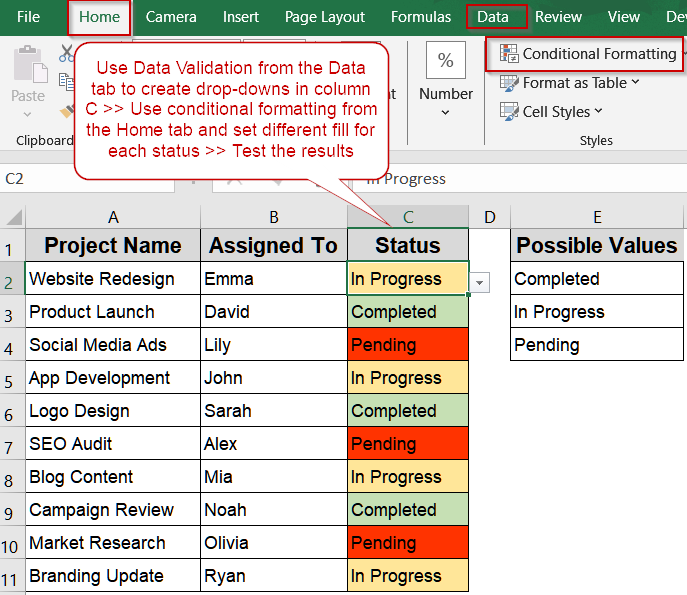
Steps to Create a Drop Down List with Color in Excel
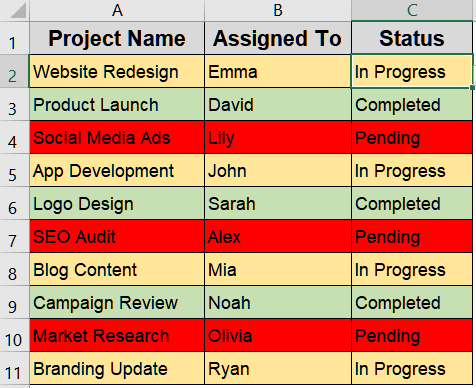
Color-coded drop-down lists help you visually track project progress, status, or performance at a glance. Each drop-down selection triggers a specific color, reducing confusion and improving productivity. We’ll use the following dataset for demonstration where we will create a drop-down list with color in the Status column:
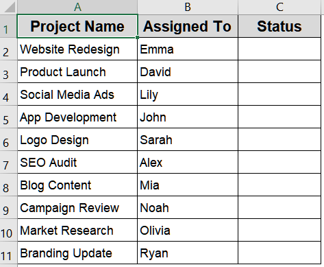
Step 1: Prepare Your Dataset
Organizing your data before you start saves time and prevents errors later. A clean layout and a dedicated list of status values make applying Data Validation and Conditional Formatting straightforward and easier to update when your workflow changes.
Steps:
➤ Open your Excel sheet containing the table above.
➤ Keep the “Status” column (C2:C11) blank initially or with current entries you wish to format.
➤ List possible status values such as Completed, In Progress, and Pending in a separate range (for example, E2:E4).
➤ Optionally, name that range as StatusList for easier reference.
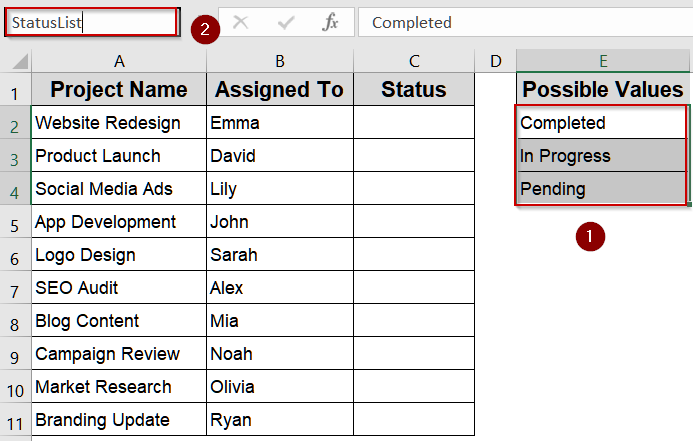
Step 2: Create the Drop-Down List
A drop-down list enforces consistent entries and speeds up data entry. Using Data Validation with either a typed list or a named range ensures everyone uses the same status labels, which is essential for accurate conditional formatting later.
Steps:
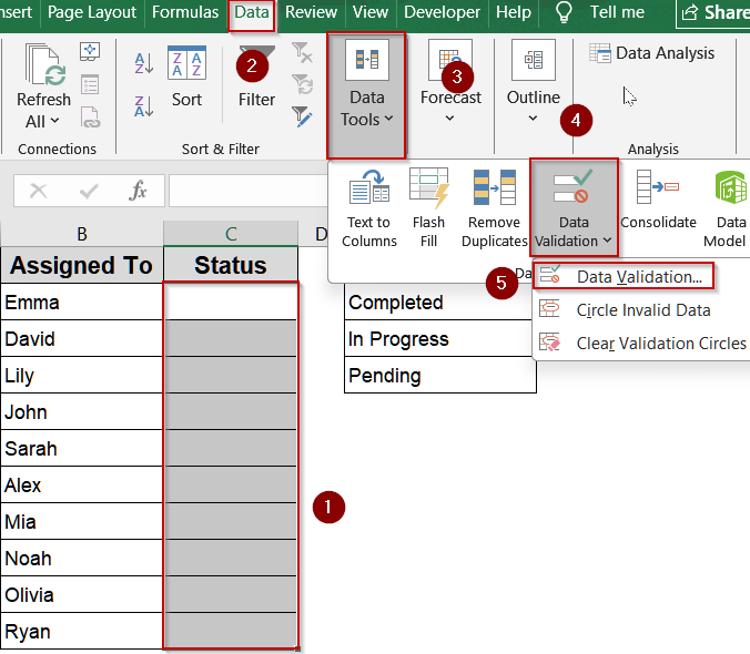
➤ Select the Status column cells (C2:C11).
➤ Go to Data tab >> Data Validation >> Data Validation.
➤ Under the Settings tab, set Allow to List.
➤ In Source box, type: Completed,In Progress,Pending
➤ Alternatively, type the following if you named your range earlier: =StatusList
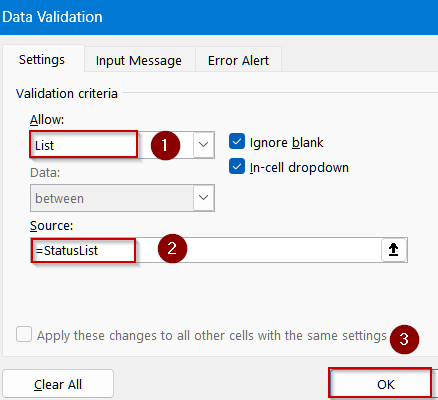
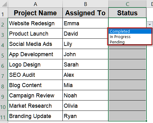
➤ Click OK. Each cell in the “Status” column now shows a drop-down arrow with these three choices.
Step 3: Apply Conditional Formatting Via Format Only Cells That Contain
Color-coding improves readability and helps you spot priorities and obstructions immediately. By creating separate rules for each status, you ensure that selections are visually distinct and consistent across the sheet. Apply this step if you only want to highlight your drop-down cells. If your goal is to highlight the full row based on your selection, skip this step.
Steps:
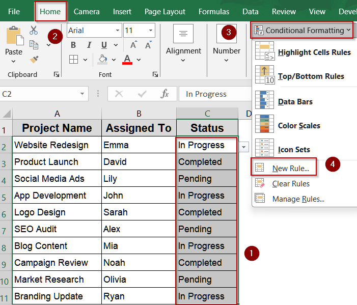
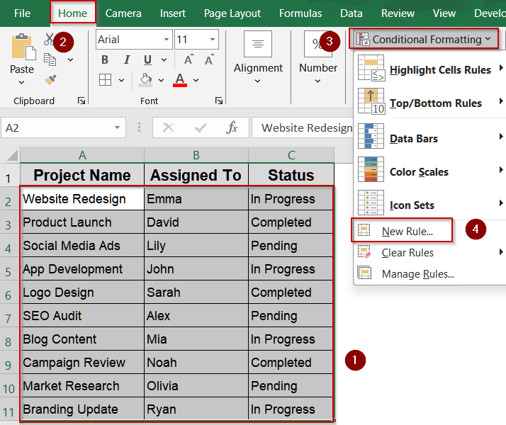
➤ Select the range (C2:C11).
➤ Go to Home tab >> Conditional Formatting >> New Rule.
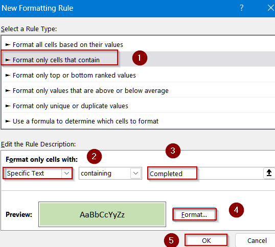
➤ Choose Format only cells that contain.
➤ In the Edit the Rule Description box, set Format only cells with option to Specific Text and type Completed next to Containing to.
➤ Click Format, choose a green fill, and click OK.
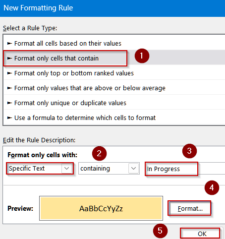
➤ Repeat this process for each status by setting a yellow fill for In Progress.
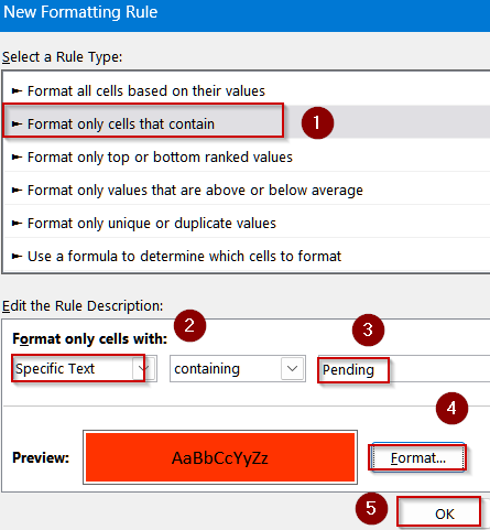
➤ Similarly, set a red fill for Pending.
Step 4: Use a Formula-Based Rule in Conditional Formatting to Highlight Full Row (Optional)
Alternatively, formula-based rules let you apply the same logic to entire rows or use dynamic references, which is useful when your workbook grows or when formatting depends on multiple cells. This approach scales better for larger tables and row-level highlighting.
Steps:
➤ Select A2:C11 again.
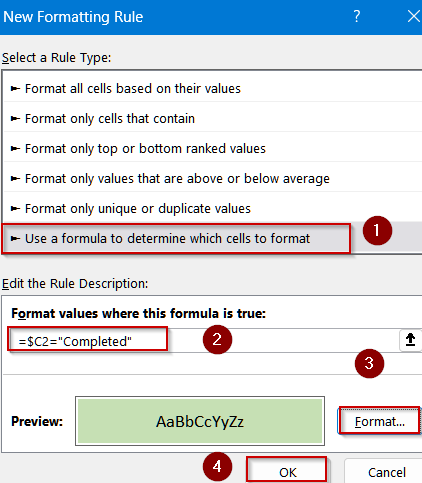
➤ Go to Conditional Formatting >> New Rule >> Use a formula to determine which cells to format.
➤ For the status Completed, type this formula:
=$C2="Completed"
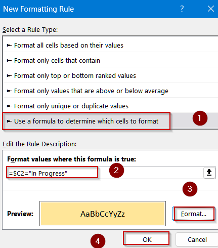
➤ For the status In Progress, type this formula:
=$C2="In Progress"
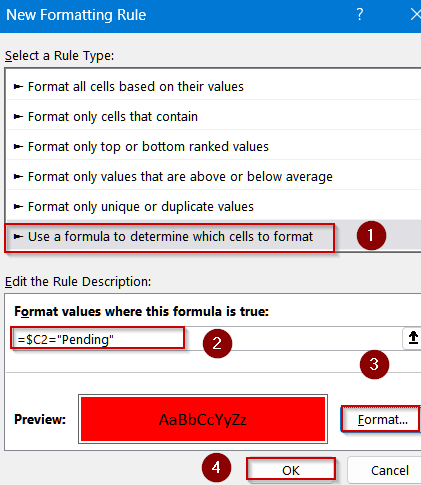
➤ For the status Pending, type this formula:
=$C2="Pending"
➤ Click Format, set your desired color, and click OK for each.
Step 5: Test the Drop-Down List
Testing confirms everything works as intended and helps you catch typos or range errors before sharing the sheet. Quick checks also show whether rules apply correctly to new rows or when values are changed.
Steps:
➤ Click any cell in the “Status” column.
➤ Choose Completed, In Progress, or Pending from the drop-down.
➤ Watch as the cell automatically changes color (green, yellow, or red).
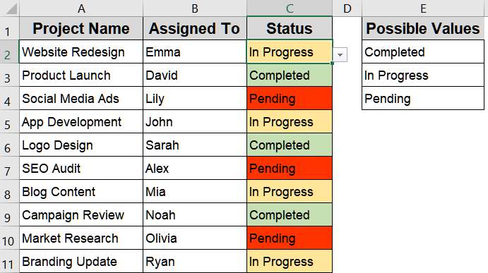
➤ Furthermore, if you have used the Use a formula technique, then your output will highlight the entire row.
Downloadable Resources
Get our practice workbook or necessary files that we have worked with to prepare this article.
Frequently Asked Questions
Can I apply different colors to multiple options in one drop-down cell?
Yes, by creating multiple Conditional Formatting rules. Each rule should target one specific text value (like “Completed” or “Pending”) and apply a unique fill color to visually distinguish between those options easily.
Why isn’t my drop-down list changing color after I select an option?
Check your Conditional Formatting formulas and ensure the text values exactly match your drop-down options, including spaces and capitalization. Also, confirm that the formatting range covers all cells containing the drop-down.
Can I color entire rows instead of just drop-down cells in Excel?
Yes, select your full dataset before applying Conditional Formatting. Then use a formula like =$D2=”Completed” to ensure the entire row color changes based on the selected drop-down status value.
Do these color-changing drop-down lists work in Excel Online?
Yes, Excel Online supports both Data Validation and Conditional Formatting. However, some complex formula-based or icon-based formatting options available in desktop Excel may not work perfectly in the web version.
Wrapping Up
In this tutorial, you learned how to create an Excel drop-down list with color to make your spreadsheets more interactive and visually intuitive. From simple Data Validation lists to advanced formula-based formatting, these techniques let you transform plain data into dynamic, easy-to-understand visuals that improve productivity and clarity. Feel free to download the practice file and share your feedback.