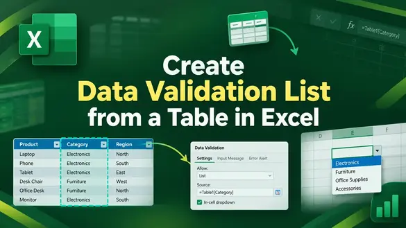

Creating a data validation list from a table in Excel helps you build drop-down menus that expand automatically when new items are added. Unlike static lists, a table-based validation list stays current as your data grows which is perfect for managing product names, departments, or categories dynamically.
In this article, you’ll learn how to create a data validation list from a table using four effective methods. Each one keeps your dropdown lists flexible and automatically updated. Let’s get started.
Steps to create data validation list from a table in Excel:
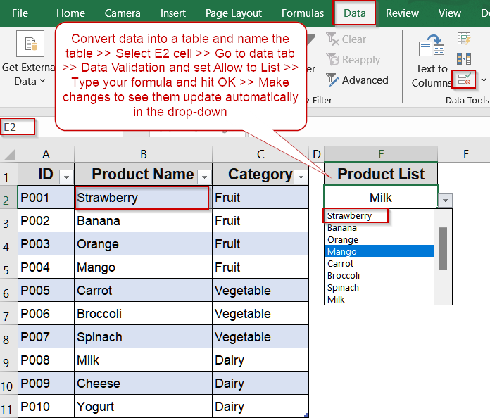
➤ Select the dataset (A1:C11) and press Ctrl + T to convert it into an Excel table.
➤ Click anywhere in the table, go to the Table Design tab, and name it ProductsTable.
➤ Go to the Data tab and choose Data Validation.
➤ In the dialog box, choose List under the “Allow” dropdown.
➤ In the Source box, enter: =INDIRECT(“ProductsTable[Product Name]”)
➤ Click OK. Your dropdown list will now pull values from the Product Name column of your table.
Create a Dynamic Drop-Down Using a Table Range
When you need a straightforward dropdown that lists all items from a column without relying on table references or named ranges, using a fixed range is the easiest approach. By selecting a sufficiently large range to cover future entries, you can ensure your dropdown works even as new items are added. This method is simple, compatible with all Excel versions, and avoids structured reference issues.
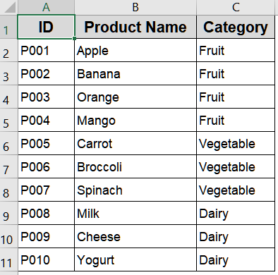
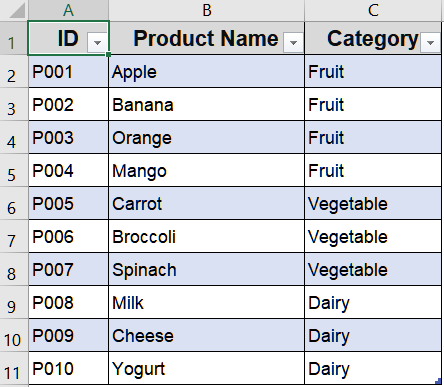
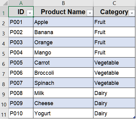
We’ll use the following dataset with product names and their categories:
Steps:
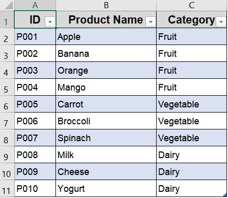
➤ Select the dataset (A1:C11) and press Ctrl + T to convert it into an Excel table.
➤ Select the cell where you want your dropdown to appear (say, E2).
➤ Go to the Data tab and choose Data Validation.
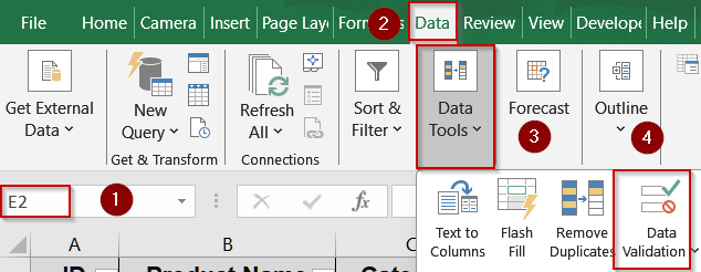
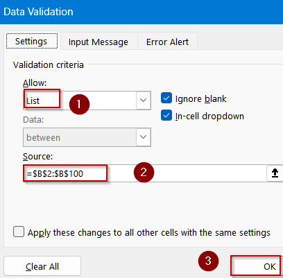
➤ In the dialog box, choose List under the “Allow” dropdown.
➤ In the Source box, type:
=$B$2:$B$100
➤ Click OK.
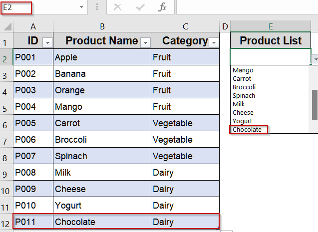
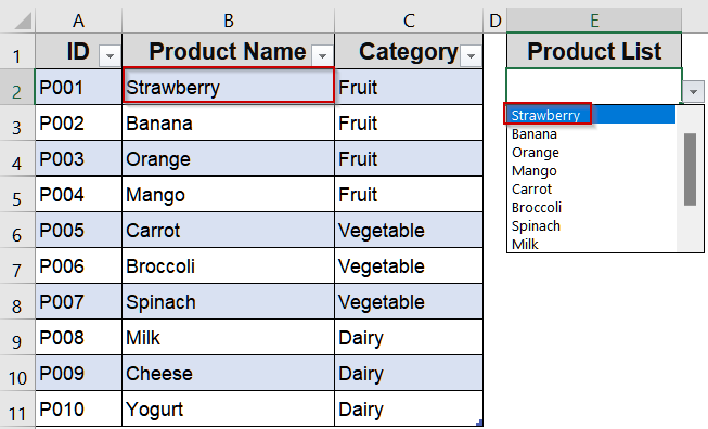
Your dropdown will now list all product names from the table and will expand automatically when new items are added to the Product Name column.
Apply the INDIRECT Function for Flexible Table References
If you manage multiple tables or frequently rename your data sources, the INDIRECT function gives you more control. It helps link a dropdown to a table column indirectly, so you can easily adapt the reference later without redoing your list.
Steps:
➤ Select the dataset (A1:C11) and press Ctrl + T to convert it into an Excel table.
➤ Click anywhere in the table, go to the Table Design tab, and name it ProductsTable.
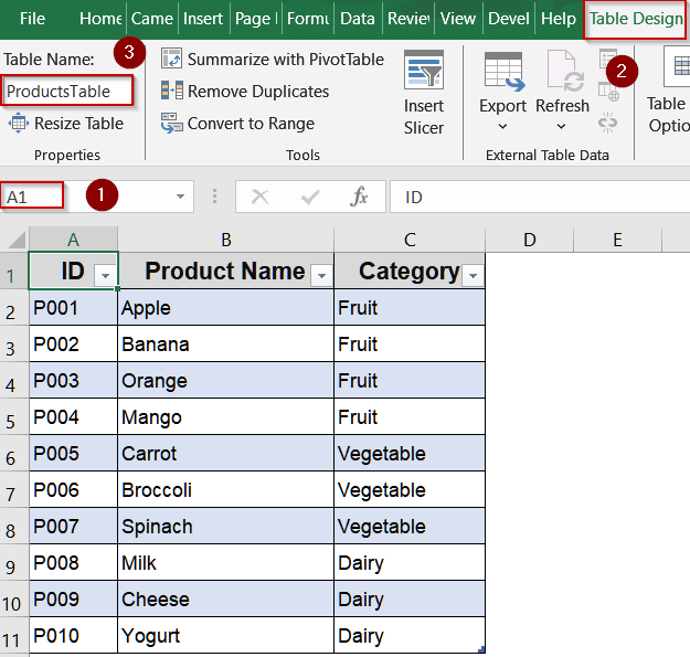
➤ Go to the Data tab and choose Data Validation.
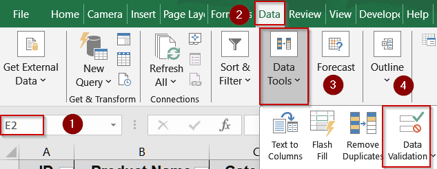
➤ In the dialog box, choose List under the “Allow” dropdown.
➤ In the Source box, enter:
=INDIRECT("ProductsTable[Product Name]")
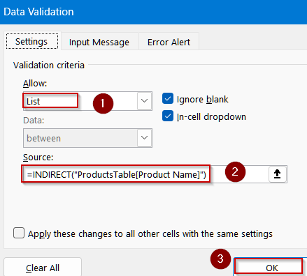
➤ Click OK.
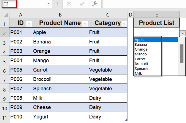
Your dropdown list will now pull values from the Product Name column of your table. If you ever rename your table or move it, just update the text in quotes without needing to rebuild the entire validation list.
Auto-Update List Using the Spill Range in Modern Excel
For Excel 365 and Excel 2021 users, dynamic arrays make dropdown creation faster and more flexible. The spill range feature lets you reference a full column from a table so new items appear instantly in your validation list.
Steps:
➤ Format your dataset as a table by pressing Ctrl + T .
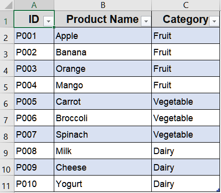
➤ Now, suppose your product names are in cells B2:B11.
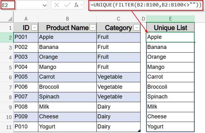
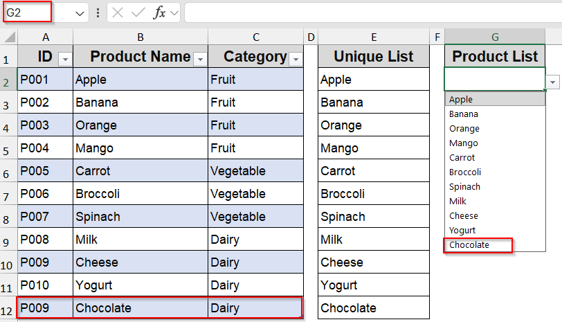
➤ In another cell, say E2, enter:
=UNIQUE(FILTER(B2:B100,B2:B100<>""))
This creates a dynamic spill list of all product names (and removes blanks).
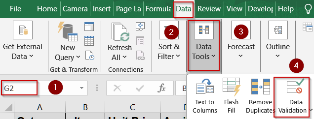
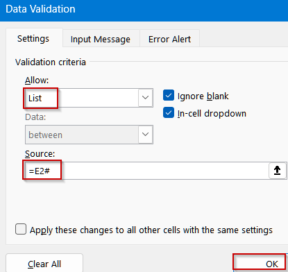
➤ Select the dropdown cell (for example, G2) and go to to Data tab >> Data Validation >> List.
➤ In the Source box, type:
=E2#
➤ Then click OK.
Now your dropdown will update instantly whenever you add or remove items in the Product Name column.
Use Named Ranges to Create a Drop-Down List Using Formulas tab
When working with data across multiple sheets or managing long lists, maintaining dropdowns can get tricky. Named ranges offer a clean and portable solution that makes managing and updating your lists much easier. By linking the dropdown to a named range, you ensure it stays connected to your source data. Any changes made to the table such as adding or removing products will automatically reflect in your dropdown, making it a reliable option for dynamic lists.
Steps:
➤ Select the dataset (A1:C11) and press Ctrl + T to convert it into an Excel table.
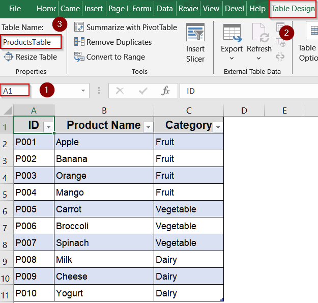
➤ Click anywhere in the table, go to the Table Design tab, and name it ProductsTable.
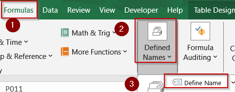
➤ Go to Formulas tab >> Click on Defined Name under the drop-down.
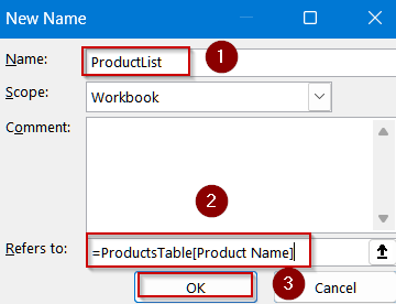
➤ In the Name box, type: ProductList
➤ In the Refers to box, enter:
=ProductsTable[Product Name]
This references the Product Name column from your table.
➤ Click OK to save the named range.
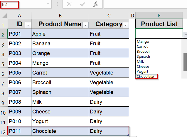
➤ Select the cell where you want the dropdown (for example, E2).
➤ Go to Data >> Data Validation >> List.
➤ In the Source box, type:
=ProductList
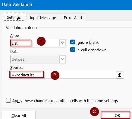
➤ Click OK.
Downloadable Resources
Get our practice workbook or necessary files that we have worked with to prepare this article.
Data Validation from Table.xlsx
Frequently Asked Questions
Why is it better to use a table when creating a data validation list in Excel?
Creating an Excel data validation list from a table is better because tables automatically expand or shrink as data changes. You don’t need to manually update cell references every time new items are added.
Can I use more than one column to create a single dropdown list in Excel?
Yes, you can. By combining multiple table columns using dynamic formulas like UNIQUE, FILTER, or CHOOSE, you can display values from different categories in a single Excel dropdown, ensuring flexible and comprehensive list options.
What happens to my dropdown if I delete or rename items in the source table?
When you delete or rename rows in the source table, the Excel data validation list from table automatically updates. This ensures your dropdown list always reflects only the existing, valid table entries.
Can I use structured table references for data validation lists across different sheets?
Yes. Structured references can be used anywhere in the workbook. You can easily refer to another sheet’s table by typing the full table name and column header in your validation Source box formula.
How can I modify or remove an existing Excel data validation list from table?
To edit or remove the dropdown, select the validated cell, go to Data >> Data Validation, then adjust the Source reference or choose Clear All to instantly remove the applied validation rule completely.
Wrapping Up
In this tutorial, you learned how to create an Excel data validation list from a table using four practical methods including fixed ranges, spill ranges, named ranges and the INDIRECT function. Each approach ensures your dropdown stays dynamic, saving time and keeping your spreadsheets clean and efficient. Feel free to download the practice file and share your feedback.