Organizing your data in Google Sheets involves more than simply the numbers. It also involves how well you display them. Using the Merge Cells feature is a simple but effective method to enhance the appearance of your Google Sheet. Combining two or more adjacent cells into a single, bigger cell is possible through cell merging. Merging cells in Google Sheets is helpful when making headers, titles, or section dividers that must span several columns or rows. In this article, we will explain the many methods of cell merging in Google Sheets and when to use each of them.
What Does Merge Cells Mean in Google Sheets?
Combining two or more cells into a single, bigger cell is called cell merging. This can be useful when:
- You want to centre a title across columns.
- In a table, you are formatting the headings.
- Your data organization needs to look cleaner.
Merging Columns in Google Sheets
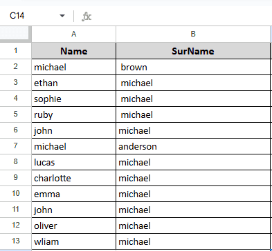
When you want to create a clean layout in Google Sheets, such as when you want to combine column cells into a single title or header across a row, you can merge columns. It improves the readability of your spreadsheet. Let’s consider the following dataset, where all entries are in the default format now.
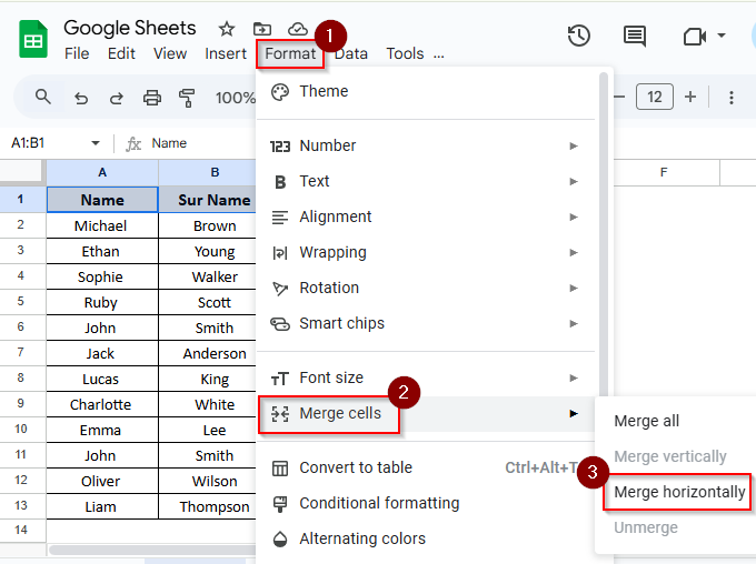
➤ Select A1 and B1 if you want to merge the first two columns in the first row.
➤ Click on the Format menu in the top toolbar.
➤ Hover over Merge cells in the dropdown.
➤ Choose Merge horizontally from the list of options.
➤ A pop-up message will appear because it will preserve only the leftmost value of the column.
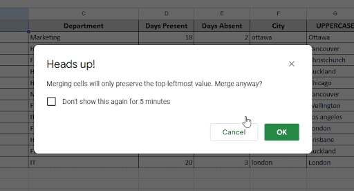
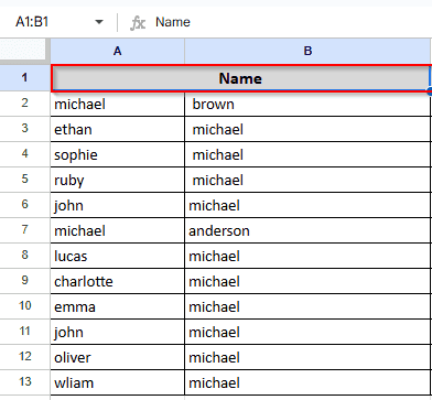
➤ Click OK, and then you can see the result. Two columns are merged into one.
Merging Cells in Google Sheets Without Losing Data
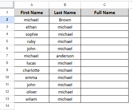
In Google Sheets, the standard “Merge cells” option only keeps the information in the top-left cell; all other content is removed. But don’t worry! You can use a formula to merge the contents of several cells into one, preserving all the information. Let’s consider the following dataset, where all entries are in the default format now.
➤ Click on cell C2 and type this formula
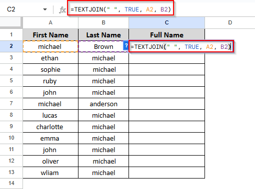
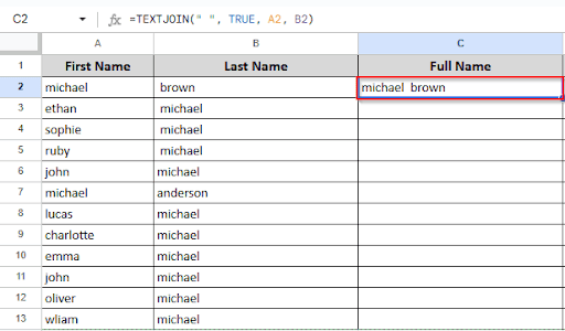
➤ Press ENTER and you will see the result.
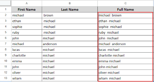
➤ Click and drag down to apply the formula to the rest of the column.
Merging Rows in Google Sheets
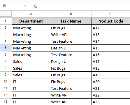
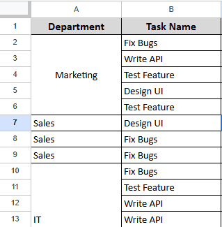
Merging rows in Google Sheets is a simple way of organizing your spreadsheet by combining cells in a single column vertically. It is useful for creating large labels, clear section names, or simply making your data appear more readable and organized. Let’s consider the following dataset, where all entries are in the default format now.
To merge rows, you have to follow these steps:
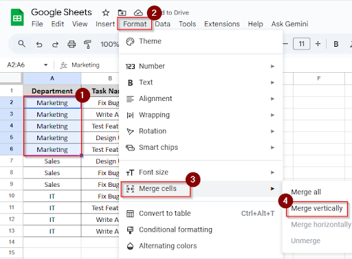
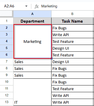
➤ Select A2 to A6 (the Marketing cells).
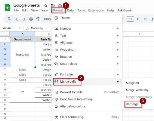
➤ Click on Format in the top menu bar.
➤ Hover over Merge cells in the dropdown menu.
➤ Then select “Merge vertically.”
➤ A pop-up message will appear because it will preserve only the leftmost value of the column.
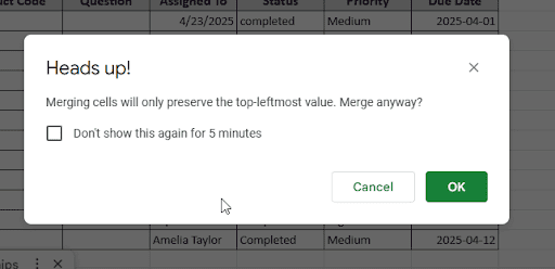
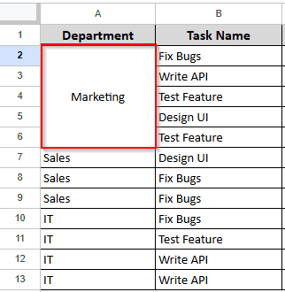
➤ Click OK, and then you can see the result. Rows are merged into one.
Shortcut for Merging Cells in Google Sheets
Merging cells is an excellent way to arrange your data, whether you’re using Google Sheets regularly. You can use it to create headers, labels, or just to make your data look better. However, you can save time by using a keyboard shortcut to merge cells quickly instead of continuously navigating through menus. What you have to do is:
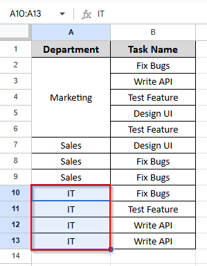
➤ Select the cells A10 to A13
➤ Use the keyboard shortcut, the shortcut is:
- Windows/Chromebook: Alt + O + M
- Mac: Option + O + M
This opens the Merge cells menu instantly.
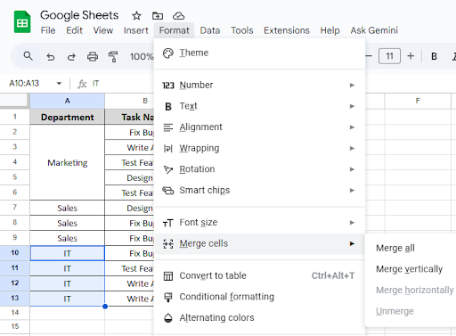
➤ After pressing the shortcut, you’ll see merge options like:
- Merge all (combines everything into one big cell)
- Merge vertically (across rows)
➤ Just click the one you want—or press the arrow keys and hit Enter to select.
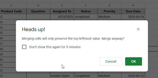
➤ A pop-up message will appear because it will preserve only the leftmost value of the column.
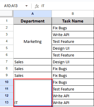
➤ Click OK, and then you can see the result. Using the keyboard shortcut, rows are merged into one.
Unmerging Cells in Google Sheets
In Google Sheets, merging cells is an excellent way to combine data or format titles, but what if you need to separate the combined cells later? Unmerging cells is elementary and just requires a few clicks, whether you’re editing a shared sheet or have simply changed your mind about it. What you have to do is:
➤ Click on the cell A2 to A6 that’s been merged.
➤ Click Format in the menu bar.
➤ From the dropdown, hover over Merge Cells to reveal more options.
➤ Click Unmerge option.
➤ Cells are now back to individual cells.
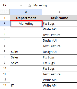
The content from the merged cell will stay in the top-left cell, and all the other cells will become empty again. You can now edit or reuse each cell individually.
Frequently Asked Questions
Why can’t I merge cells in Google Sheets?
Cells from separate rows and columns cannot be merged. Connected cells are only merged. If the cells are protected, you can’t merge, and frozen columns or rows cannot be merged. Also, when the sheet is in view-only mode, you can’t merge cells in Google Sheets.
Why is the merge option grayed out?
This can happen if:
- You’re trying to merge non-adjacent cells
- The cells are protected or locked
- You’re in a filtered or frozen section
- You don’t have editing permissions
Concluding Words
Although merging cells in Google Sheets isn’t difficult, it can greatly simplify and organize your spreadsheet. Whether you’re working on a project, organizing data for a team, or simply making your sheet appear a little prettier, you have to understand how to merge and unmerge cells. If you accidentally merge something, it’s simple to correct to unmerge.