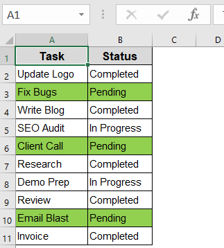
Sometimes you need more than just numbers. Whether you’re managing categories, tracking statuses, or sorting names, Excel makes it easy to highlight cells based on text values. Conditional formatting allows you to visually emphasize keywords or phrases automatically, no manual searching needed.
In this article, we’ll show you multiple ways to highlight text-based cells in Excel using built-in rules, custom formulas, and even partial match techniques. These methods help you spot trends, flag issues, or simply make your spreadsheets easier to scan.
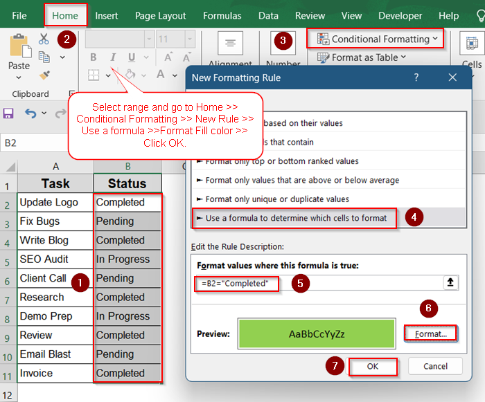
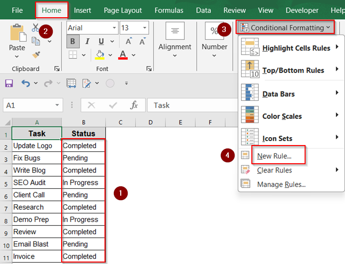
Steps to highlight cells based on text in Excel :
➤Select desired range .
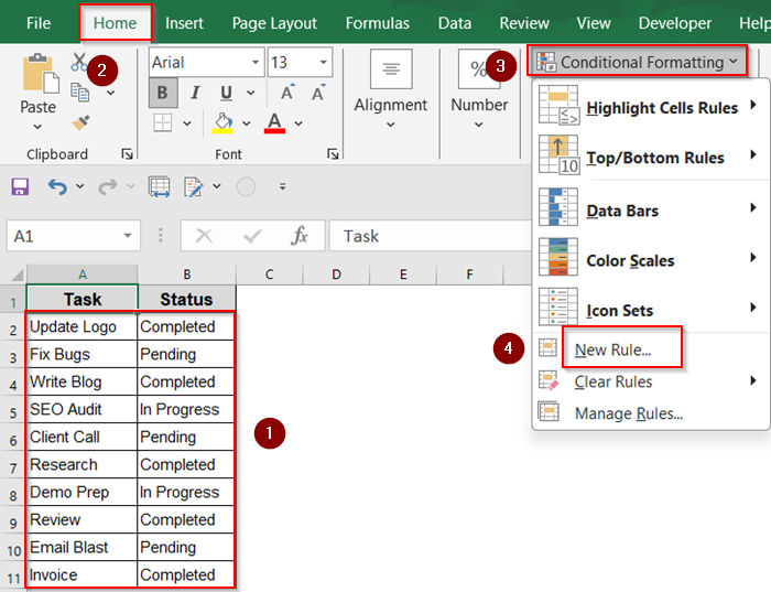
➤ Go to Home >> Conditional Formatting >> New Rule.
➤ Choose Use a formula and enter the formula: =B2=”Completed”
➤ Format using Fill color >> Click OK.
Apply Color to Cells That Match Specific Text
If you’re working with specific terms like “Pending” or “Completed,” Excel’s built-in conditional formatting makes it easy to highlight exact matches in your dataset without writing formulas. Perfect for status tracking and quick data scans.
Steps:
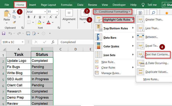
➤ Select the range where you want to apply highlighting (e.g., B2:B11 for the “Status” column).
➤ Go to Home >> Conditional Formatting >> Highlight Cells Rules >> Text that Contains.

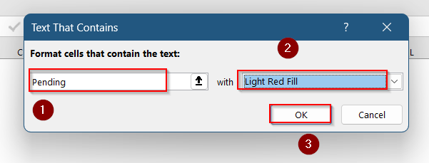
➤ Type the exact word (e.g., Pending).
➤ Choose a formatting style (e.g., light red fill).
➤ Click OK.
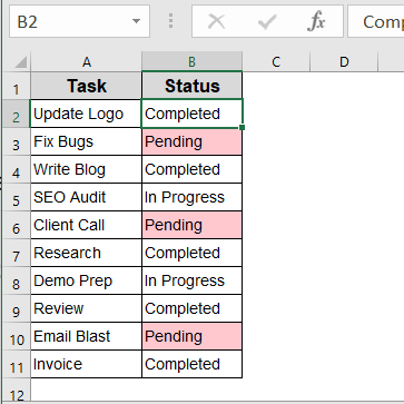
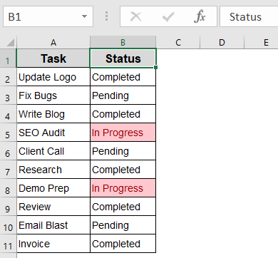
Now all cells with the word “Pending” will be highlighted.
Format Cells That Contain Partial Match
Use this method when your data contains phrases, and you want to flag any cell with a partial word like “Progress.” It’s useful for text that varies slightly but shares a consistent keyword.
Steps:
➤ Select your range (e.g., B2:B11).
➤ Go to Home >> Conditional Formatting >> Highlight Cells Rules >> Text that Contains.
➤ Type Progress (not the full phrase).
➤ Choose your format and hit OK.
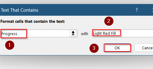
This will highlight any cell that includes the word “Progress,” such as “In Progress“.
Use a Formula to Match Full Text Precisely
For pinpoint control, especially when dealing with dynamic data or variable row structures, use a formula that matches the text exactly. This ensures only perfect matches are formatted which is ideal for review workflows or approvals.
Steps:
➤ Select the range you want to format (e.g., B2:B11).
➤ Go to Home >> Conditional Formatting >> New Rule.
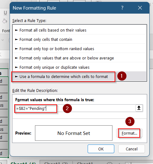
➤ Choose Use a formula to determine which cells to format.
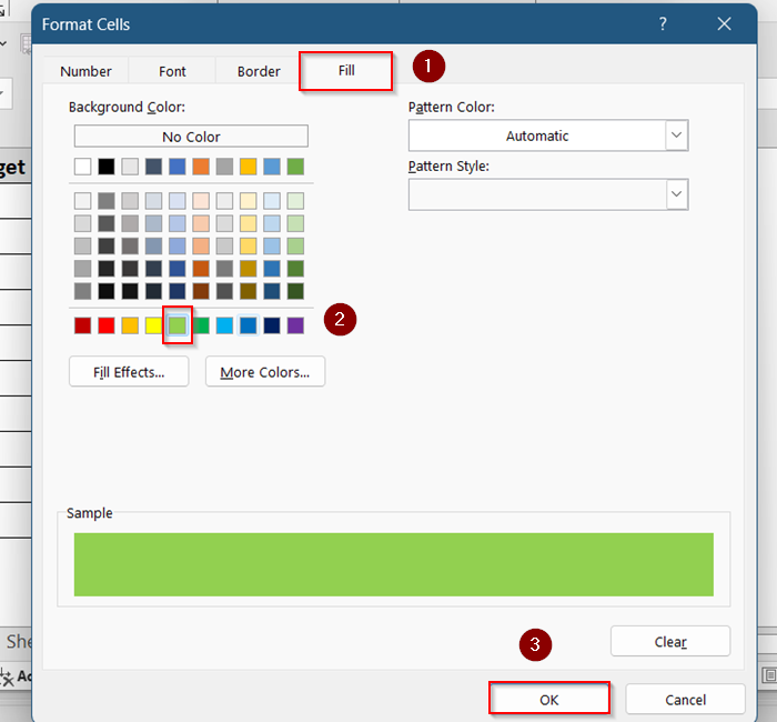
➤ Enter the formula:
=B2=”Completed”
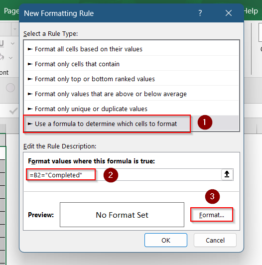
➤ Click Format, pick a fill color (e.g., green), and click OK.
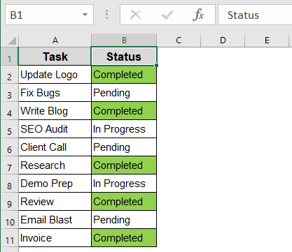
All cells that exactly match “Completed” will be highlighted.
Highlight Rows Based on Text in One Column
Want to highlight the entire row if the status column says “Pending”? Use a formula that locks the column reference but lets the row change.
Steps:
➤ Select the full range (e.g., A2:B11).
➤ Go to Home >> Conditional Formatting >> New Rule.
➤ Choose Use a formula to determine which cells to format.
➤ Enter this formula:
=$B2=”Pending”
➤ Click Format, choose a Fill color, and press OK.

Now, each row with “Pending” will be fully highlighted.
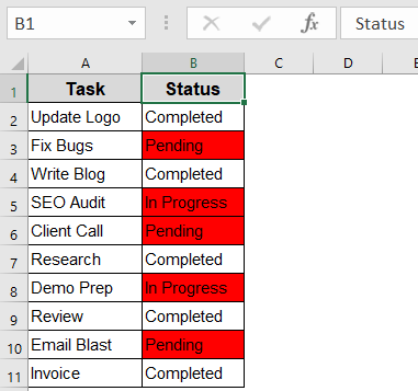
Mark Cells That Do Not Contain Certain Text
This method is perfectIf you’re filtering out unwanted entries like everything except “Completed”. It visually flags cells that are missing expected text, making it easier to track incomplete or problematic records.
Steps:
➤ Select the target range (e.g., B2:B11).
➤ Go to Home >> Conditional Formatting >> New Rule.

➤ Choose Use a formula to determine which cells to format.
➤ Enter this formula:
=B2<>”Completed”
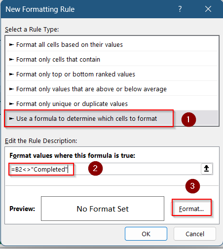
➤ Click Format, select a fill color, and click OK.
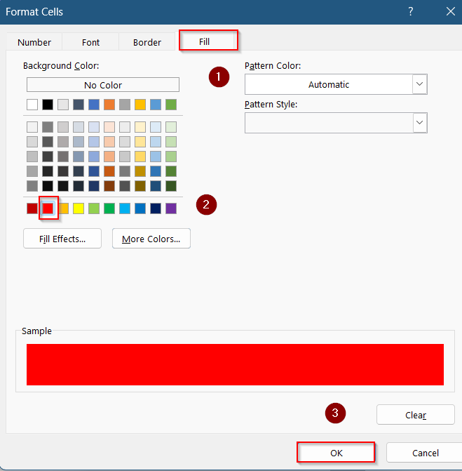
This will highlight all cells that do not contain “Completed”.
Frequently Asked Questions
Can I highlight cells based on multiple text values?
Yes, use a formula like =OR(B2=”Pending”, B2=”In Progress”) to highlight cells matching either of the two values.
Can I make the highlight case-sensitive?
Not with the default rules. But you can use a formula like =EXACT(B2,”Completed”) for a case-sensitive match.
Will this work in Excel for Mac?
Yes, all Conditional Formatting methods described here also work in Excel for Mac, although menu placements may slightly vary.
Can I highlight part of the cell text?
Yes, Excel’s built-in Text that Contains rule works even if the word is part of a longer phrase.
How do I remove conditional formatting?
Go to Home >> Conditional Formatting >> Clear Rules, and choose whether to clear from the selection or entire sheet.
Wrapping Up
In this tutorial, we learned multiple ways to highlight cells in Excel based on text including exact match, partial match, and even row-level formatting. These tools can greatly enhance the readability and usability of your spreadsheet. Feel free to download the practice file and share your feedback.