How to Color Scatter Plot by Group in Excel (2 Useful Ways)

Scatter plots in Excel are useful for visualizing relationships between variables. Coloring the scatter plot based on groups, such as regions or categories, highlights patterns or trends. Let’s say you have profit margins in certain regions compared to sales. Coloring the scatter plot by group will help you easily identify the regions with higher profit margins. This article covers both the manual way using helper columns and the VBA automation to color a scatter plot by group.

Key Takeaways

➤ First, create helper columns to group your data from the dataset.
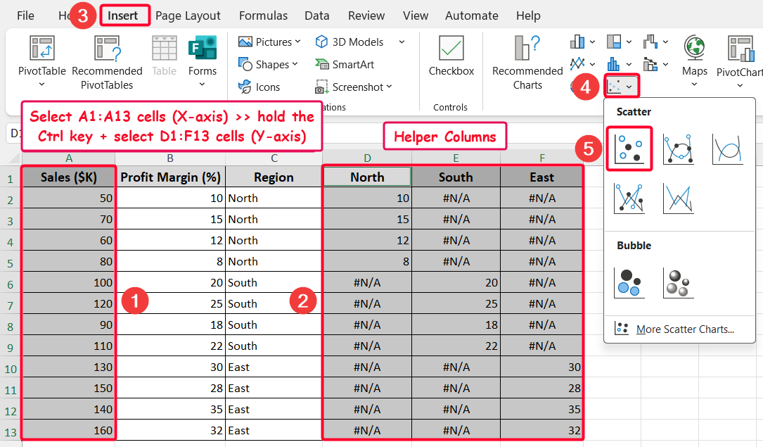
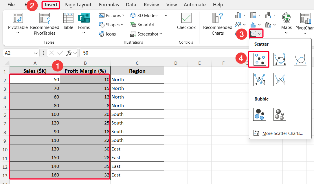
➤ Select the X-axis data, hold the Ctrl key, and then select the Y-axis data
➤ Lastly, go to the Insert tab >> choose the Scatter option from the Charts ribbon group.

In this article, you’ll get the idea of creating helper columns to split the Y-axis by group for coloring the plot, and then VBA automation to do it easily.

Download Practice Workbook

Color Scatter Plot by Group Using Helper Columns

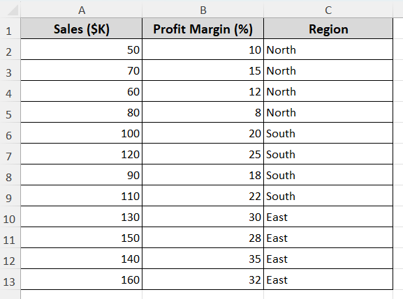
Let’s have a look at the following dataset which shows sales figures (in $K), corresponding profit margins (%), and regional classifications (North, South, East).

Now, we will classify the profit margin data based on the North, South, and East regions. That means we will split the data of the Y-axis by regions. Then, we will create a scatter plot so that the chart automatically uses different colors for each region group.

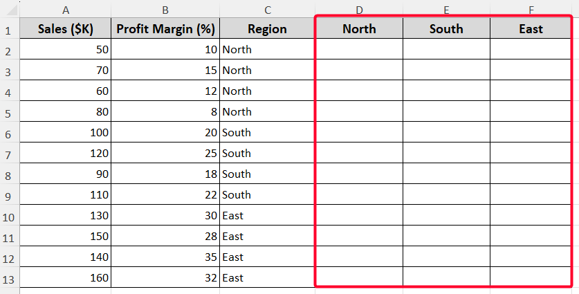
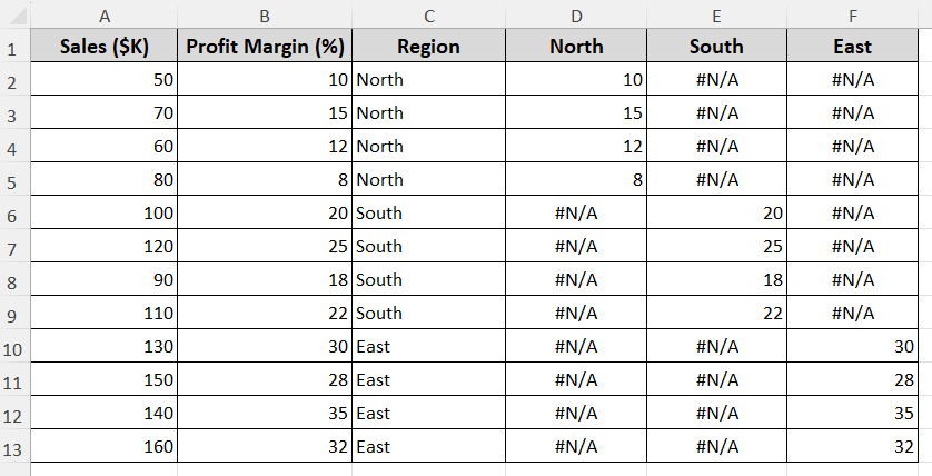
➤ At the outset, create 3 helper columns for each region, namely North, South & East.

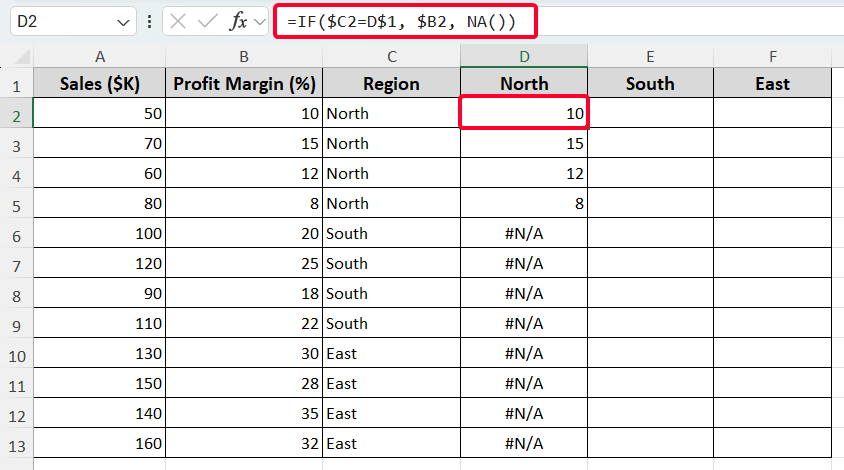
➤ In the D2 cell, enter the following formula to get the profit margin for the north region from the C2:C13 cells.

=IF($C2=D$1, $B2, NA())

The formula checks if the region in cell C2 matches the region name in cell D1 (“North”); if it does, it returns the profit margin from cell B2; otherwise, it returns #N/A.

➤ Similarly, use the following formula for the other 2 regions.

For the south region:

=IF($C2=E$1, $B2, NA())

For the east region:

=IF($C2=F$1, $B2, NA())

➤ So, the output looks like the one below.

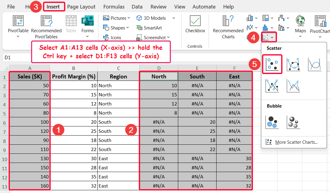
➤ Now select the A1:A13 cells (X-axis) >> hold the Ctrl key and select the D1:F13 cells (Y-axis).
➤ Lastly, go to the Insert tab >> choose the Scatter option from the Charts ribbon group.

➤ Shortly, you’ll get a scatter plot with different colors by regions with legends.

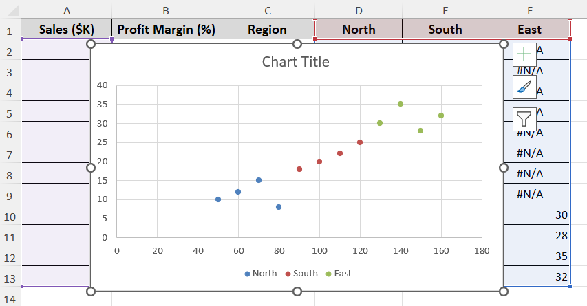
➤ Customize the created scatter plot (e.g. adjust chart title, add axis titles from the plus icon shown in the top-right corner of the chart.)

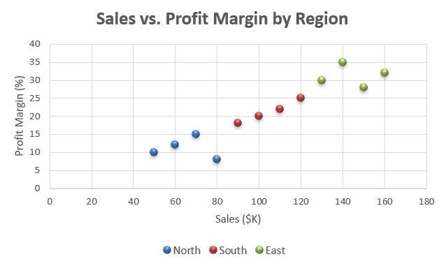
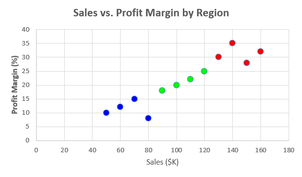
So the final output looks like the following one.

Note:
This method works for any number of groups (typically up to 255); not limited to 3 regions.

Use VBA Code

Without creating any helper columns, you can color a scatter plot by group using a simple VBA code.

➤ First select A2:B13 cells >> create a scatter plot from the Charts group of the Insert tab.

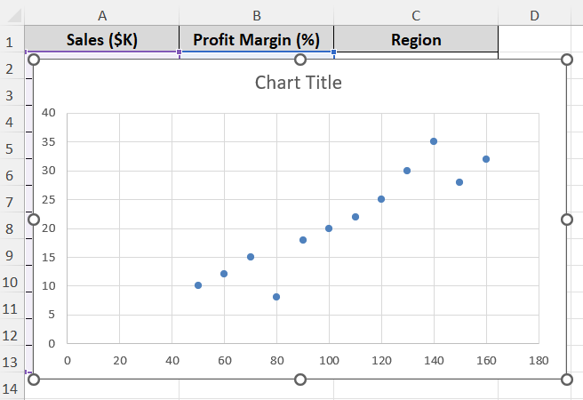
➤ After that, you will have a scatter plot with the same colors for each region.

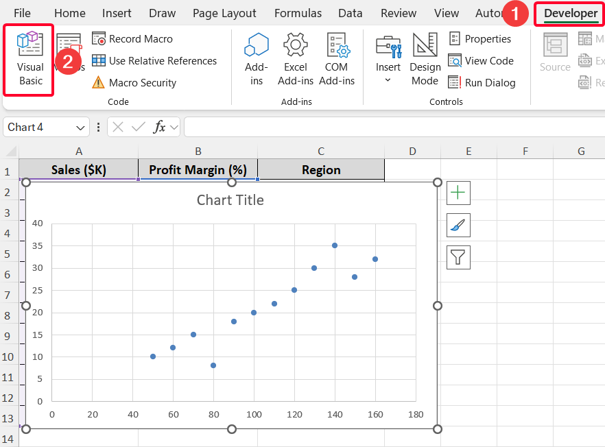
Now we will apply the VBA automation. If you’re a new Excel user and didn’t use VBA, enable the Developer tab first from the Customize the Ribbon of Excel Options.

➤ Then go to the Developer tab >> click on the Visual Basic thumbnail.

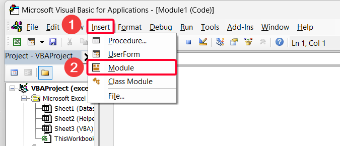
➤ Go to the Insert tab >> Module option to insert a new module.

➤ Copy the following code and paste it into the module.

Sub ColorScatterPlotByRegion()
    Dim crt As Chart, ser As Series, pnt As Point, m As Long
    Dim vRange As Range, pointColor As Long
    ' Set the chart (adjust ChartObjects(1) if needed)
    Set crt = ActiveSheet.ChartObjects(1).Chart
    Set ser = crt.SeriesCollection(1)
    ' Set the Region column range
    Set vRange = Range("C2:C13")
    ' Loop through each point
    For m = 1 To ser.Points.Count
        Set pnt = ser.Points(m)
        Select Case LCase(vRange(m).Value)
            Case "north": pointColor = RGB(0, 0, 255) ' Blue for North
            Case "south": pointColor = RGB(0, 255, 0) ' Green for South
            Case "east": pointColor = RGB(255, 0, 0) ' Red for East
        End Select
        pnt.Format.Fill.ForeColor.RGB = pointColor
        pnt.MarkerSize = 8 ' Optional: Set point size
    Next m
End Sub

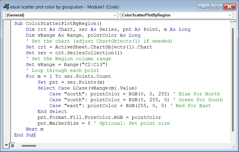
➤ Don’t forget to change the cell range of the region column and region names in your data.
➤ Run the code by pressing the F5 key.

The VBA code will produce a scatter plot with different colors for each region.

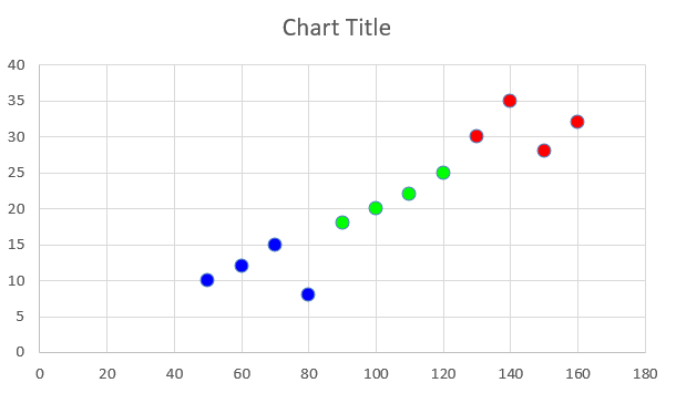
➤ Adjust the chart elements based on your requirements, and the final chart will look like the following.

Note:
This method doesn’t create the legend automatically. Here comes a handy trick: simply copy the legend from the chart created with helper columns and paste it onto the chart above.

Frequently Asked Questions

Is coloring by group in scatter limited to 3 groups?

You can use the manual method with helper columns for many groups, not just 3 regions. Excel supports up to 255 groups, so you can easily apply this to large datasets with many categories.

How do I add new groups after creating the scatter plot?

Add a new column in your data for the new group, as shown in the first method. Then right-click on the chart, choose “Select Data,” >> “Add” to include the new series. After adding the data, press OK.

Why can’t I change the color of individual points within one series?

You cannot assign unique colors to individual points within a single series by default in Excel. Therefore, you need to split the data into grouped series for group-based coloring.

Wrapping Up

This is how you can easily color a scatter plot by group in Excel with a manual method by creating helper columns, as well as VBA automation. We hope that you have enjoyed the article. Feel free to download the practice workbook and share your thoughts in the comments!

Post Views: 4