
By using a basic AVERAGE formula, Excel automatically ignores empty cells, but sometimes those cells can contain empty strings (“”) or text. In such a case, calculating the average will not be accurate. If you want to know the average value of non-blank cells, then zeros and blank cells must be removed. In this article, we will learn several ways to use formulas, built-in features, and dynamic array functions to determine the average of just non-blank cells in Excel.
Steps to average only Non-Blank cells in Excel using the AVERAGEIF function:
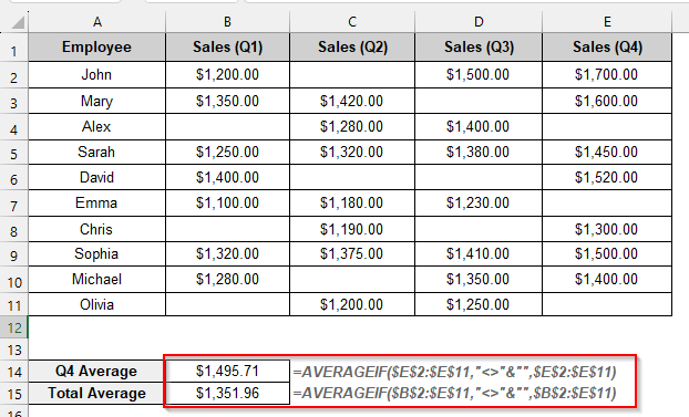
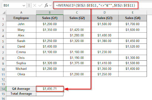
➤ Select the B14 cell and write this formula to calculate the average value of non-blank cells of Q4 sales.
=AVERAGEIF($E$2:$E$11,”<>”&””,$E$2:$E$11)
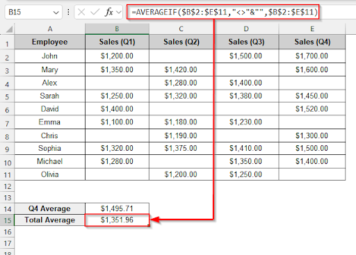
➤ To determine the overall average value of non-blank cells, choose the B15 cell and write this formula.
=AVERAGEIF($B$2:$E$11,”<>”&””,$B$2:$E$11)
In this article, we will explore various methods to average only non-blank cells in Excel. Using the AVERAGEIF function, using table totals, combining the AVERAGE function with the IF function, utilising the AVERAGEIFS function, combining the AVERAGE function with the FILTER function, and manual calculation are some methods.
Using the AVERAGEIF Function
We can determine the average of Excel’s non-blank cells by using the AVERAGEIF function. Blank cells are removed by the AVERAGEIF function using the not equal to blank condition (<>). The AVERAGEIF function determines the average of the numbers.
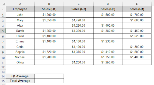
To determine the Q4 sales average and the overall sales average, let’s look at the employee sales dataset below.
Steps:
➤ Select the B14 cell and write this formula to calculate the average value of non-blank cells of Q4 sales.
=AVERAGEIF($E$2:$E$11,"<>"&"",$E$2:$E$11)
➤ Press Enter and see the average of non-blank cells of sales Q4.
➤ Select cell B15 and write this formula to find the total sales average
=AVERAGEIF($B$2:$E$11,"<>"&"",$B$2:$E$11)
➤ Enter this formula in cell B15 to see the total average value of the non-blank cells.
Combining the AVERAGE Function with the IF Function
Excel’s IF and AVERAGE functions can be combined to get the average of only non-blank cells. The AVERAGE function computes the average of the non-blank cell values after the IF function determines whether or not each cell is blank. The blank cells are then eliminated by the not equal to blank condition.
Steps:
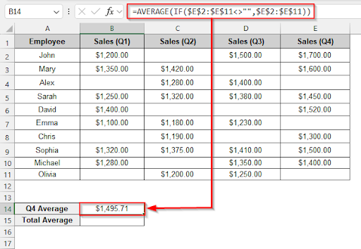
➤ Select the B14 cell and write this formula to calculate the average value of non-blank cells of Q4 sales.
=AVERAGE(IF($E$2:$E$11<>"",$E$2:$E$11))
➤ Press Enter and see the average of non-blank cells of sales Q4.
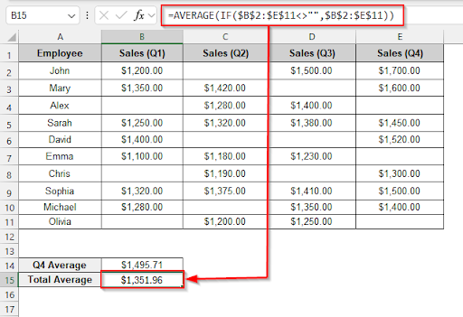
➤ Select cell B15 and write this formula to find the total sales average.
=AVERAGE(IF($B$2:$E$11<>"",$B$2:$E$11))
➤ Press Enter and see the average of non-blank cells of total sales.
Using the AVERAGEIFS Function
Excel’s AVERAGEIFS function allows us to calculate the average of only non-blank cells. It can manage multiple criteria. We need to set the range of values. Only cells that are not blank and contain numbers greater than zero will be counted by this condition (“<>“).
Steps:
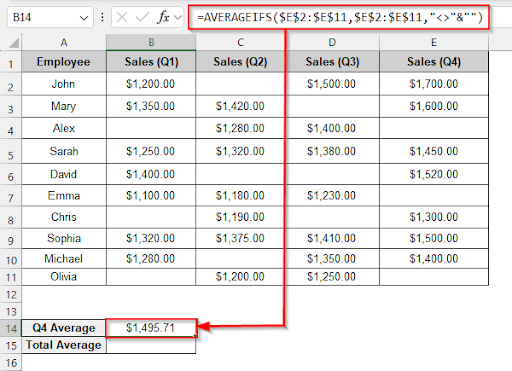
➤ Select the B14 cell and write this formula to calculate the average value of non-blank cells of Q4 sales.
=AVERAGEIFS($E$2:$E$11,$E$2:$E$11,"<>"&"")
➤ Press Enter and see the average of non-blank cells of sales Q4.
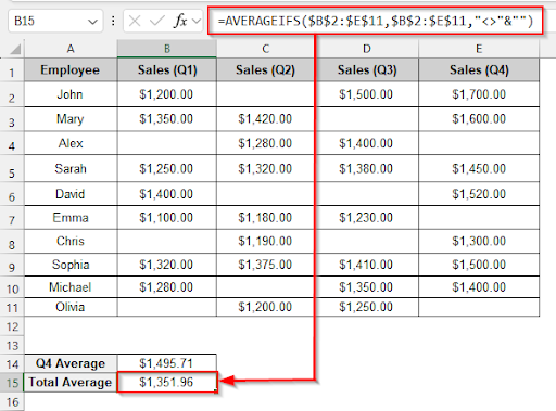
➤ Select cell B15 and write this formula to find the total sales average.
=AVERAGEIFS($B$2:$E$11,$B$2:$E$11,"<>"&"")
➤ Press Enter and see the average of non-blank cells of total sales.
Combining the AVERAGE Function with the FILTER Function
This method will remove blank cells from the dataset by combining the AVERAGE and FILTER functions. The FILTER function will filter the non-blank cells. The average of those non-blank cells will be calculated by the AVERAGE function.
Steps:
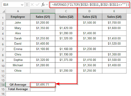
➤ Select the B14 cell and write this formula to calculate the average value of non-blank cells of Q4 sales.
=AVERAGE(FILTER($E$2:$E$11,$E$2:$E$11<>""))
➤ Press Enter and see the average of non-blank cells of sales Q4.
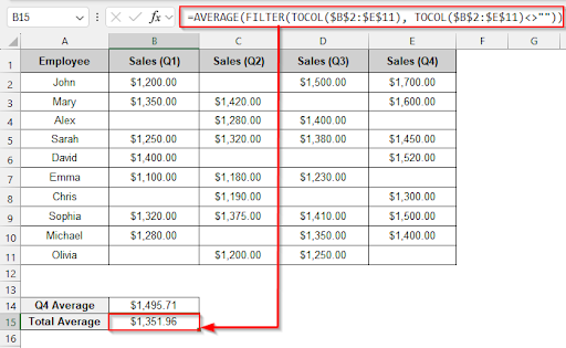
➤ Select cell B15 and write this formula to find the total sales average
=AVERAGE(FILTER(TOCOL($B$2:$E$11), TOCOL($B$2:$E$11)<>""))
➤ Press Enter and see the average of non-blank cells of total sales.
Manual Calculation
The manual calculation method means that we need to sum the non-blank cells using the SUM function, then divide by the count of those non-blank cells with the COUNT function. By doing this manual calculation, we can find the average of only non-blank cells in Excel.
Steps:
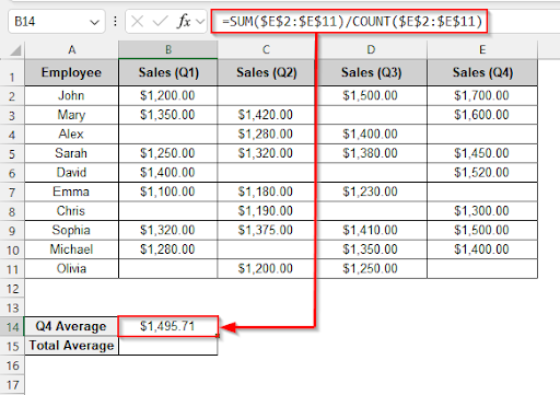
➤ Select the B14 cell and write this formula to calculate the average value of non-blank cells of Q4 sales.
=SUM($E$2:$E$11)/COUNT($E$2:$E$11)
➤ Press Enter and see the average of non-blank cells of sales Q4.
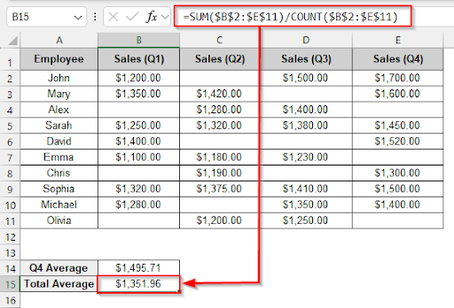
➤ Select cell B15 and write this formula to find the total sales average
=SUM($B$2:$E$11)/COUNT($B$2:$E$11)
➤ Press Enter and see the average of non-blank cells of total sales.
Using Table Totals
The table total method automatically ignores blank cells. First, we need to convert the data into a table. Then, we can use the total row option to find the average value of the data. If new data is added, the table updates dynamically.
Steps:
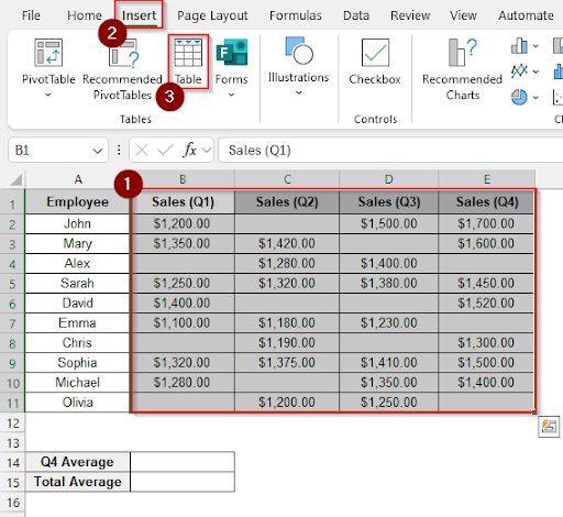
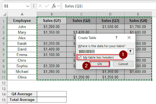
➤ Select the B1 to E11 cells and click Insert>table to create a table. In the table window, choose the “my table has headers” option and click OK.
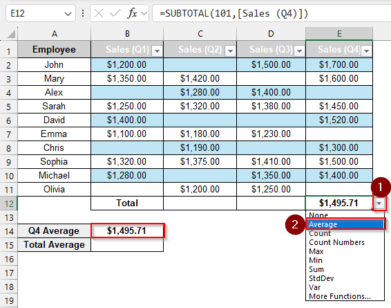
➤ Click Table Design and check the Total Row option.
![]()
➤ Now you will see the Total of the Q4 sales.
![]()
➤ Click the dropdown arrow and choose Average from the dropdown. Then you will see the Q4 sales average of non-blank cells.
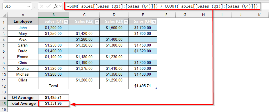
➤ To find the total average, click on cell B15 and write this formula
=SUM(Table1[[Sales (Q1)]:[Sales (Q4)]]) / COUNT(Table1[[Sales (Q1)]:[Sales (Q4)]])
➤ Press Enter and see the average of non-blank cells of total sales.
Frequently Asked Questions
Is it possible to ignore zero-value cells when calculating the average?
Use =AVERAGEIF(range, “<>0”) function to ignore zero-value cells in Excel.
Which function should I use after filtering data to calculate the average of non-blank cells?
Use the SUBTOTAL function or the AGGREGATE function to calculate the average of the non-blank cells after filtering.
Why am I facing an error while using the AVERAGEIF formula?
The AVERAGEIF formula returns an error if all the cells are blank or contain text. This formula only works with numbers.
Does Excel’s AVERAGE function ignore blank cells automatically?
Yes, the AVERAGE function will automatically ignore the blank cells and calculate the average.
Wrapping Up
In this article, we discussed six different methods that how you can average only non-blank cells in Excel, along with detailed steps. Feel free to download the practice file and share your thoughts and suggestions in the comment box. Hopefully, you will enjoy this article.