While working in excel, we may often work with datasets with blank cells. And we need to sum up values in a range based on a different column where we have some blank cells. In these cases, we use the sum if not blank criteria.
However, there are multiple methods and functions we can apply to use this criteria. The first and foremost one is the SUMIF function. Apart from the SUMIF, we will also discuss the other alternatives we can try depending on our needs.
➤ Insert the following formula in cell B13:
=SUMIF(C2:C10,”<>”,D2:D10)
➤ Tap Enter and we’ll get the result in the same cell.
Now let’s go through the step-by-step discussion.
Overview of the SUMIF Function in Excel
The SUMIF function in Excel is designed to add up values in a range that meets a certain condition.
Syntax:
=SUMIF(range, criteria, [sum_range])
➤ range → The cells where Excel looks for the condition.
➤ criteria → The rule that decides which cells to include.
➤ sum_range → The numbers to add up.
Example:
=SUMIF(A2:A11, "Laptop", C2:C11)
![]()
Using SUMIF Function to Sum Non-Blank Cells Values in Excel
To sum values in a range when its corresponding cells are not blank, we can simply use the SUMIF function. It allows us to use a non-blank value (“<>”) in the criteria argument of the function. It means the formula will avoid the blank cells and only sums the values from the specific range by following that.
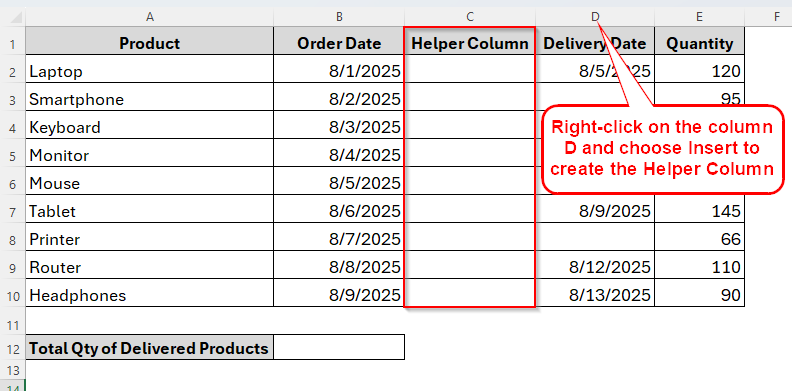
Now let’s assume we’ve a dataset containing a list of some Products including their Order date, Delivery date and Quantity. If any product is not delivered yet, the corresponding cell in column C is empty.
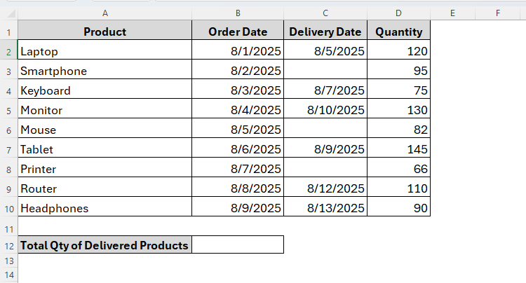
So, we’re going to count the total quantity from column D only if the delivery date is not blank in column C. For this, we’ll simply apply the SUMIF function as follows.
Steps:
➤ Go to the cell where you want the result. In our dataset, we choose B12.
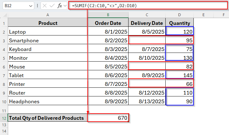
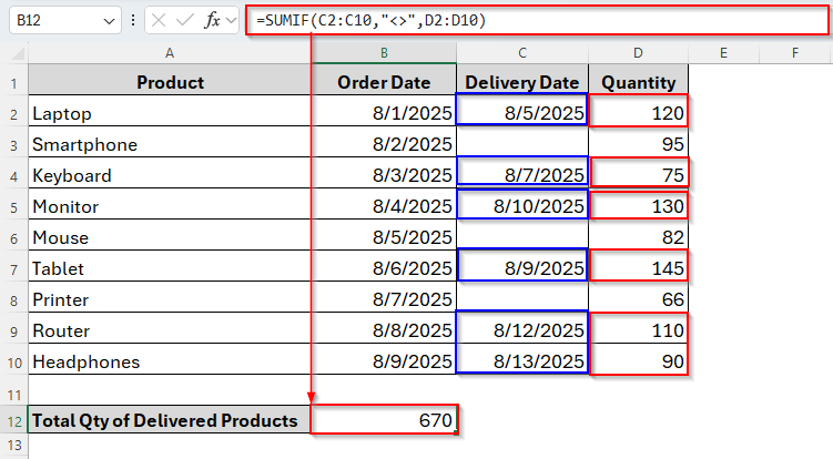
➤ Now in the cell B12, type the following formula:
=SUMIF(C2:C10,"<>",D2:D10)
➤ Tap Enter and the formula will return the sum of the quantities for only those cells where there’s a delivery date as the image shows below:
Applying Helper Column with TRIM Function to Sum Non-Blank Cells
Sometimes, the SUMIF function may not be able to sum accurately when some cells are blank in the dataset. It is because the blank cells are often not truly empty. They may contain data as a space character.
So, this can create problems because Excel doesn’t always recognize them as blank. To fix this, we can create a helper column and use both the TRIM and LEN functions. Here, the TRIM function will remove spaces, while the LEN function is likely to count the number of characters from the cell. If the LEN function shows 0, it means that the cell is truly empty.
And now we’ll create a helper column beside the Delivery Date column to remove the space and return the number of characters in each cell. After that we can apply the SUMIF function to count the total quantity from Column D. Let’s explore how it works.
Steps:
➤ Insert the Helper Column beside the Delivery Date column.
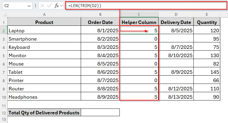
➤ Next, use the TRIM and LEN functions in cell C2 as follows:
=LEN(TRIM(D2))
➤ Press Enter and drag the AutoFill handle down to the cell C10. By doing so, it will generate a number like 5 in our dataset when the cell has data or it will show 0 if the cell is truly blank.
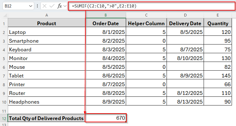
➤ Now we can sum the total quantities of the delivered products with the SUMIF function with the greater than 0 criteria. So, apply the following formula in cell B12:
=SUMIF(C2:C10,">0",D2:D10)
➤ Hit Enter. And this ensures that only truly filled Delivery Dates are counted.
Alternative Formulas to Sum Only Non-Blank Cells in Excel
Besides the SUMIF function, there are some other different functions in Excel that also allow us to sum with If not blank criteria. So, in this part of the article, we’ll discuss some of those common functions so you can choose and apply the best fit for your dataset.
Combining SUM & FILTER Functions
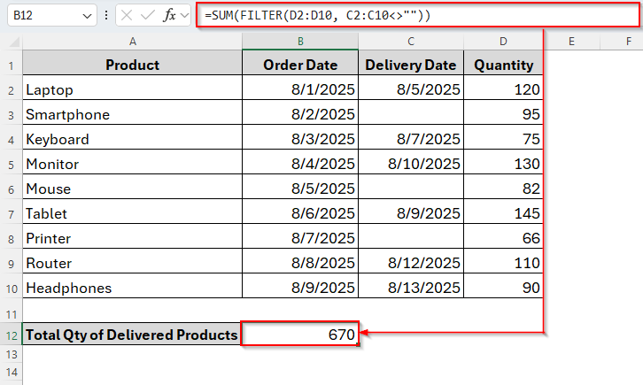
This is a modern and cleaner way to sum values in Excel while skipping blank cells. With the FILTER function, it removes all the blank cells and then the SUM function adds up the values from the remaining cells.
This method is very useful if you work with a larger dataset and need an easy and clean formula without Helper Column. Unlike the SUMIF or SUMPRODUCT functions, this is more flexible, and can handle more complex conditions. To use this function, below are the steps to follow:
Steps:
➤ Click on the cell B13 and insert the following formula:
=SUM(FILTER(D2:D10, C2:C10<>""))
➤ Tap Enter and it will add up the total quantity of the delivered products only.
Using the SUMPRODUCT Function
Another most common sum function in Excel is the SUMPRODUCT. It can also sum values if cells are blank. It works by multiplying two or more ranges and then summing up the results. This function is extremely useful in older versions of Excel where FILTER is not available.
Steps:
➤ Insert the formula in cell B13 as follows:
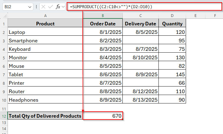
=SUMPRODUCT((C2:C10<>"")*(D2:D10))
Here, (C2:C10<>””) creates an array of TRUE/FALSE based on whether the cell is blank. Then multiply it with Quantity and only keep the non-blank rows.
➤ Then press Enter. The formula will generate the sum of the quantity skipping the blank cells from column C.
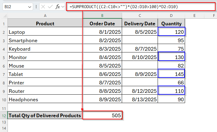
However, this method is so powerful because it works even if you want to add more conditions later. Suppose you want to sum Quantity only if Delivery Date is not blank and Quantity is greater than 100. There’re totally two different criteria and here’s how we can use it:
Steps:
➤ Similarly to the previous method, insert the formula in cell B13 as below:
=SUMPRODUCT((C2:C10<>"")*(D2:D10>100)*D2:D10)
➤ Hit the Enter key. And as you can see in the image below, it totals the numbers only up to 100 and also ignores the blank cell from column C while summing up.
Using the SUMIFS Function
Last but not least, the SUMIFS function would be the simplest way to add values in Excel. With this, fortunately, we can also skip blank cells. It is very useful for quick calculations and is easier to understand compared to SUMPRODUCT or FILTER. However, unlike FILTER, it is less flexible for multiple advanced conditions.
Steps:
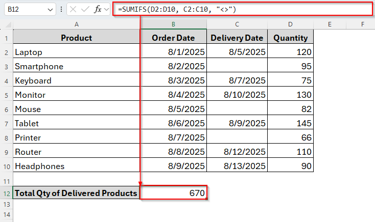
➤ Select and type the following formula in B13.
=SUMIFS(D2:D10, C2:C10, "<>")
➤ Press Enter and the result is here.
Frequently Asked Questions
Can I Sum with If Not Blank Criteria for Cells Across Multiple Columns?
Yes, you can. But you just have to apply the SUMIFS function instead of SUMIF. With SUMIFS, you can easily use multiple conditions as follows:
=SUMIFS(D2:D10, C2:C10,”<>”, B2:B10,”<>”)
What if the blank cells are caused by formulas returning “” (empty text)?
Sometimes, Excel treats “” as non-blank. So, the generic if not blank criteria may not work here. To solve that, use the following formula instead:
=SUMPRODUCT((LEN(C2:C10)>0)*(D2:D10))
Concluding Words
Summing values only if a cell is not blank is a very common requirement in Excel. Whether you use SUMIF, SUM + FILTER, or SUMPRODUCT, all methods can get the job done. However, if you want the simplest way, just use the SUMIF. But if you are on Excel 365, go for SUM + FILTER for a cleaner approach. Other methods are also handy and suitable for different purposes.