By default, the VLOOKUP function in excel searches for a value in the first column of a table range and returns the result from another column to the right. And I would say, this is the biggest minus point of this function. The VLOOKUP function cannot lookup left and therefore, it requires the lookup column to be the first in the range. Typically, we use Helper Column to solve this.
But sometimes the lookup value may not be in the first column and so, we need to rearrange columns without moving them physically. Well, in these cases, we can combine VLOOKUP with CHOOSE function to rearrange data virtually. Let’s see how we can do it at a glance.
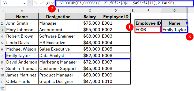
➤ Enter the Employee ID in cell F3.
➤ Now insert the following formula in cell G3:
=VLOOKUP(F3, CHOOSE({1,2}, $D$2:$D$11, $A$2:$A$11), 2, FALSE)
➤ Press Enter and we’ll get the result in the same cell.
Now, further on this tutorial, we’ll explore multiple methods to use VLOOKUP along with the CHOOSE function with examples. So, let’s dive in.
Overview of the Excel CHOOSE Function
Before we jump into the tutorial, let’s discuss the CHOOSE function in short. Basically, the CHOOSE function in Excel returns a value from a list based on the position or index you specify. It’s useful for quickly slecting values from fixed options or combining with other functions like VLOOKUP for more advanced lookups.
➤ Syntext
CHOOSE(index_num, value1, [value2], [value3], …)
Here,
Index_num: The position number (between 1 and 254)
Value 1: The first value to choose
[value2], [value3], …: Optional arguments to choose from
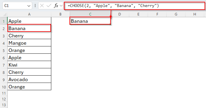
➤ Example
=CHOOSE(2, "Apple", "Banana", "Cherry")
Here, index_num = 2 means pick the 2nd item. From the list, the 2nd item is “Banana”. And as we can see in the image, the result is also Banana.
Using VLOOKUP with CHOOSE Function for a Single Criterion
As we mentioned earlier, one of the key limitations of the VLOOKUP function is that it cannot look to the left. But the CHOOSE function allows us to virtually reorder columns, so we can lookup values in columns to the left without moving any data.
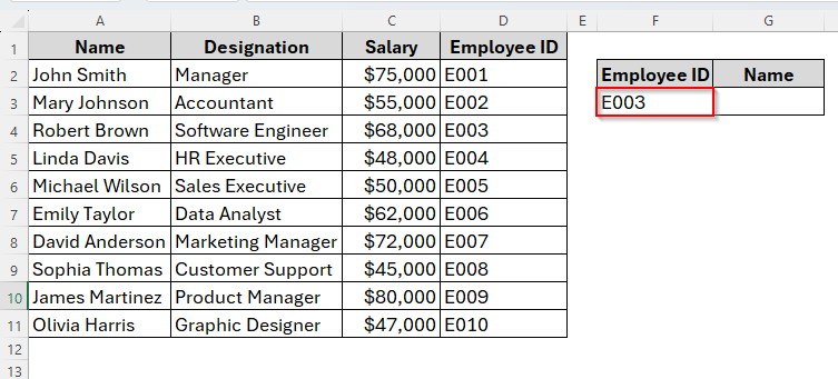
For example, below we have a list of Employees with their Employee ID in column D and Name in Column A.
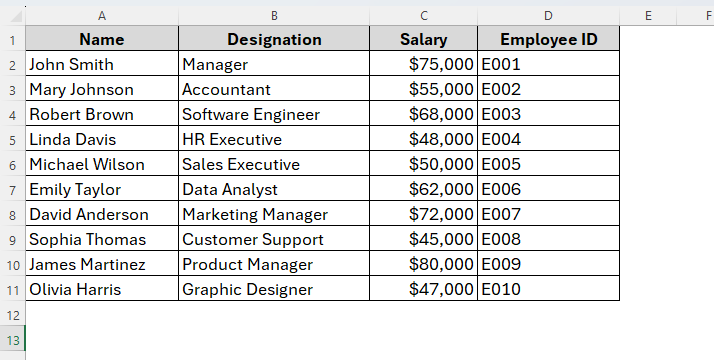
Normally, the VLOOKUP function cannot find the Name when the lookup value is Employee ID as the Name column is to the left. But using the CHOOSE function, we can simply solve this problem. Here’s how it goes.
Steps:
➤ Under Employee ID in Column F, insert the ID number in cell F3.
➤ Now select the cell where you want the result and type the formula as follows:
=VLOOKUP(F3, CHOOSE({1,2}, $D$2:$D$11, $A$2:$A$11), 2, FALSE)
➤ Hit the Enter key and here we go.
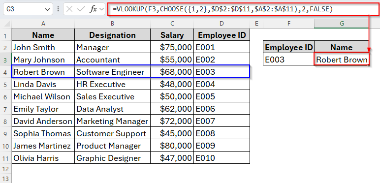
We’ve got the employee name Robert Brown according to his ID.
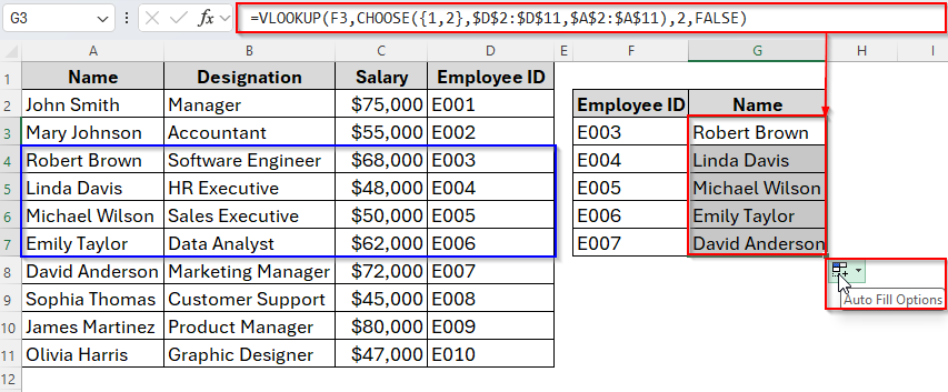
➤ Now, if you want multiple results, just insert the employee ID and drag down the AutoFill Handle from Column G3. It’ll automatically generate the result as follows.
Using VLOOKUP with CHOOSE Function for Two Criteria
Now that we know how to combine VLOOKUP with CHOOSE function with single criteria, let’s jump into two criteria. Suppose, we have to find an employee’s salary when we already know both their designation and Employee ID. Let’s see how it works.
Steps:
➤ Type the first condition in cell G2 and the second condition in cell G3. In cell G4, next to the Salary, we’ll get the required result.
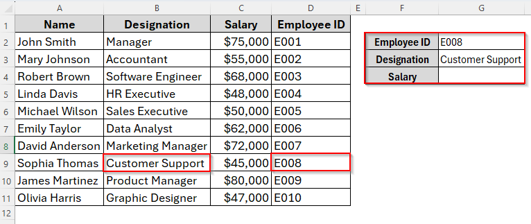
➤ Once we have the criteria, insert the formula as follows:
=VLOOKUP(G2&G3,CHOOSE({1,2},$D$2:$D$11&$B$2:$B$11,$C$2:$C$11),2,FALSE)
➤ Press Enter and the result will be shown as the image shows below.
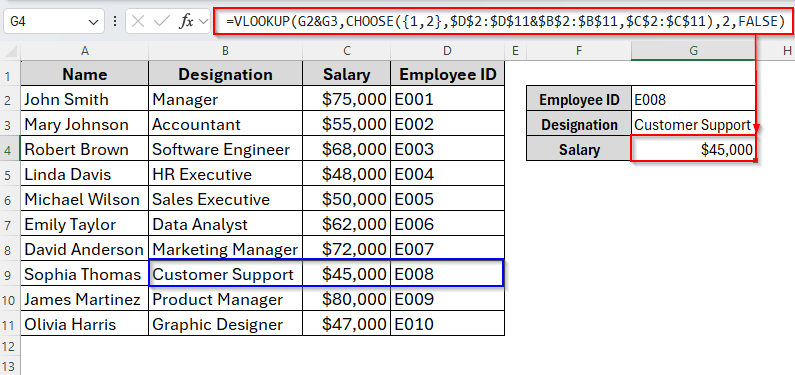
Here, G2&G3 joins the two conditions into one lookup key. Then, CHOOSE({1,2},$D$2:$D$11&$B$2:$B$11,$C$2:$C$11) creates a virtual table where the first column is the combined ID and Category, and the second column is the value to return. After that, the 2 means we want the second column from the CHOOSE output. And finally, FALSE ensures an exact match.
Using VLOOKUP with CHOOSE Function for Three Criteria
Now, we’ll combine VLOOKUP with CHOOSE function for three criteria. Let’s assume, we will find an employee’s Name when you know their Designation, Salary, and Employee ID. And the value to return is in cell G5.
Steps:
➤ To begin with, enter the three criteria in cell G2, G3, and G4.
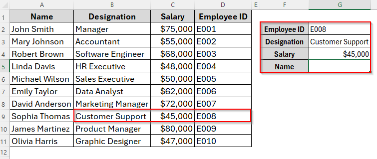
➤ Then in cell G5, type the following formula:
=VLOOKUP(G2&G3&G4,CHOOSE({1,2}, D$2:$D$11&$B$2:$B$11,$C$2:$C$11),2,FALSE)
➤ Press Enter and the result will appear as follows.
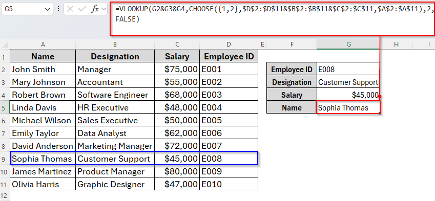
In cell G5, we have the name Sophia Thomas based on the Employee ID, Designation, and Salary.
Using VLOOKUP with CHOOSE Function for More Than Three Criteria
When it comes to more than three criteria, unfortunately the previous VLOOKUP + CHOOSE method won’t work. We’ll have to approach different functions like AVERAGE + IF.
This method is useful when you need to summarise or group data by custom combined conditions. Therefore, it works great if we need to match more than three criteria, or criteria that aren’t next to each other in the table.
In our given example, let’s assume that we’ll create a summary showing salary by Designation and first letter of Employee ID. Below are the steps to follow to do so.
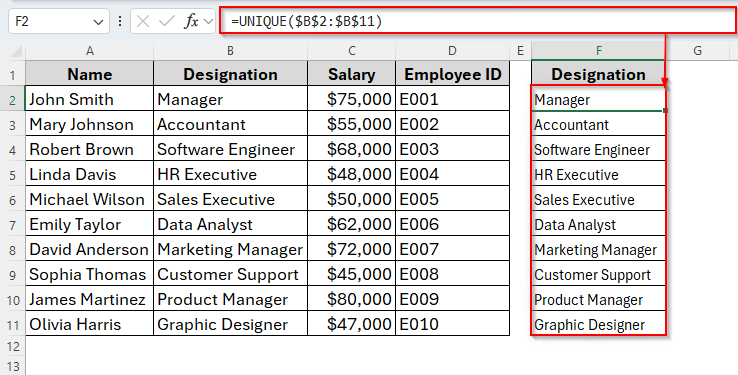
➤ Firstly, create a blank table in Column F.
➤ Then, in cell F2, type:
=UNIQUE(B2:B11)
➤ Press Enter and drag the AutoFill Handle down to cell F11. This returns unique values from column B.
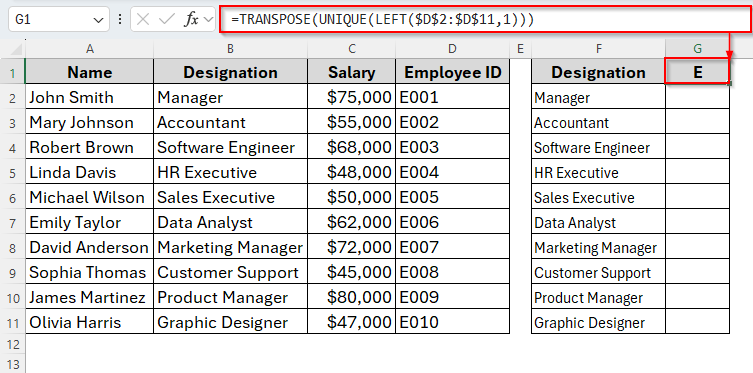
➤ Now in cell G1, apply the following formula:
=TRANSPOSE(UNIQUE(LEFT($D$2:$D$11)))
➤ Tap Enter and it will list unique first letters of Employee IDs horizontally. But as in the given example, all Employee IDs start with the letter E, we’ll only get E in cell G1 after applying the formula.
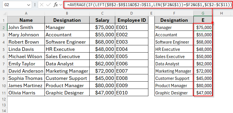
➤ Now in cell G2, insert the formula as below:
=AVERAGE(IF(LEFT($B$2:$B$11&D$2:D$11
➤ Hit Enter and it will show the salary of each employee based on designation.
Frequently Asked Questions
Why Should I Combine VLOOKUP with CHOOSE Function?
First of all, the CHOOSE function can build a virtual dynamic table through the VLOOKUP formula. Therefore, the function can lookup values based on multiple criteria and also can search to the left by reordering the columns within the function.
Is CHOOSE better than INDEX-MATCH?
These two are different functions and solve different problems in Excel. Here, INDEX-MATCH is faster on large datasets, but CHOOSE is more intuitive for creating virtual tables.
Concluding Words
That’s how you can combine VLOOKUP with the CHOOSE function in Excel to work around limitations and create more flexible lookups. From single-condition lookups to multi-criteria summaries, this combination can be a real time-saver, especially if you’re working in a version of Excel that doesn’t have XLOOKUP.
With just a bit of creativity, you can turn two simple functions into a powerful lookup tool for almost any scenario.