For summarizing large datasets, a Pivot Table is a handy tool. However, a common problem is how to update a Pivot Table when new rows of data are added to the source. Manually creating a new Pivot Table every time is a time-consuming task. In this article, we will show you several methods to add new rows of data to your Pivot Table easily. Here, we will cover a few different methods, from simple manual updates to more advanced solutions.
To add rows in a Pivot Table in Excel, here is one simple solution by changing the data source.
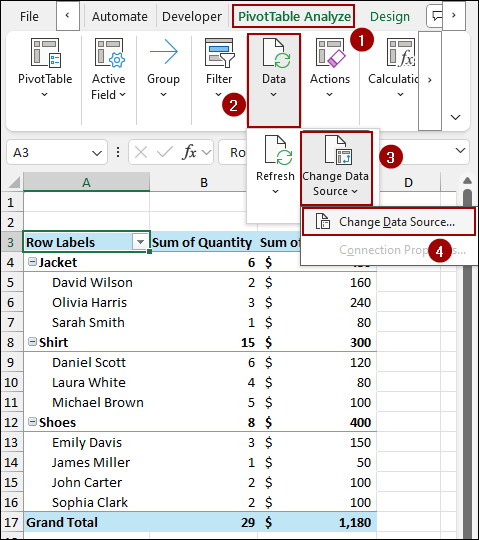
➤ Go to PivotTable Analyze > Data > Change Data Source.
➤ In the Change PivotTable Data Source dialog box, update the range to include your new rows.
➤ Click OK, and the Pivot Table will display data including new rows.
Using Change Data Source Tool
This is a method for manually updating your Pivot Table after adding new data. It involves simply expanding the range of the source data.
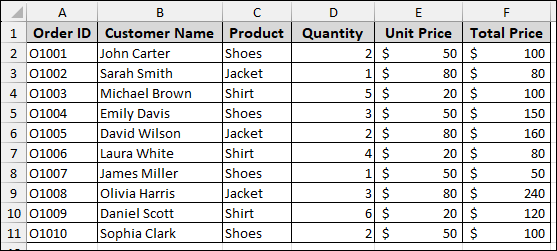
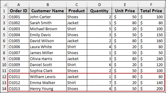
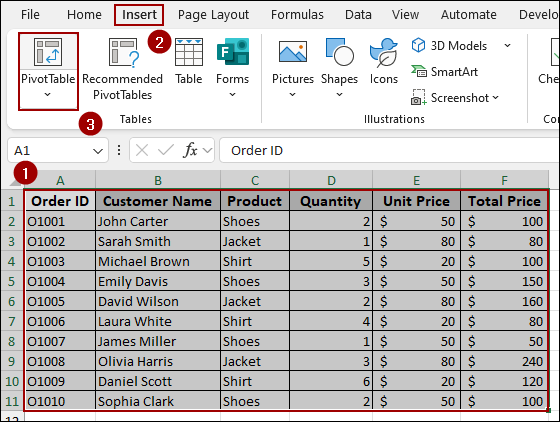
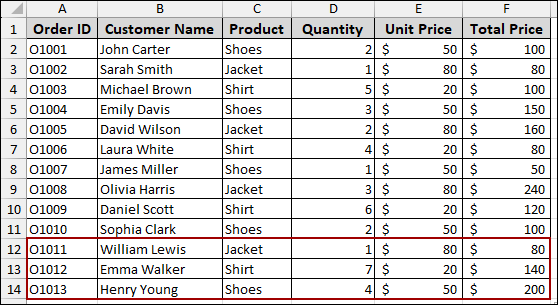
Suppose we have a dataset containing Sales Order details.
Now, we will create a Pivot Table with the dataset.
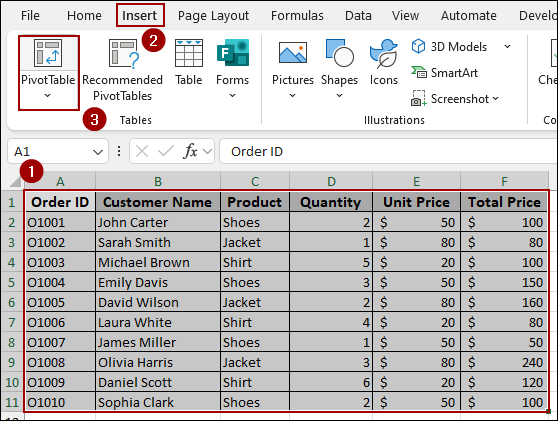
➤ Select the whole dataset and click Insert > PivotTable.
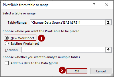
➤ In the new dialog box, choose New Worksheet and click OK.
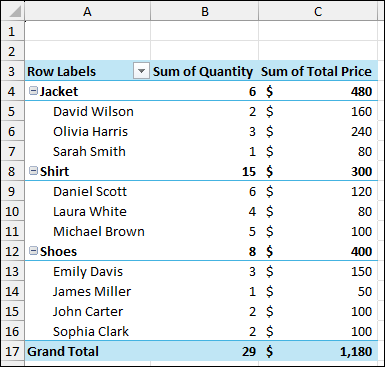
As a result, the Pivot Table will be created.
Now, let’s add some new rows of orders in the source sheet.
Coming back to the Pivot Table sheet, you will see that your Pivot Table hasn’t automatically updated to include this new data. Here is how you can manually adjust the source.
➤ Go to PivotTable Analyze > Data > Change Data Source.

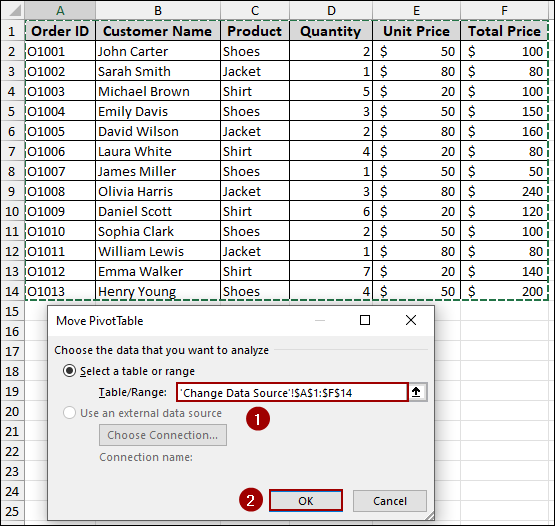
The Change PivotTable Data Source dialog box will appear. Here, you will see the current range in the Table/Range field.
➤ Update the range to include your new rows. For instance, if the original range was A1:F11 and you added data to row 14, change it to A1:F14.
➤ Click OK.
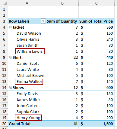
This way, the Pivot Table will now include the new data, and the values will be updated accordingly.
Inserting Rows in the Source Data Table
This is the most dynamic and efficient method for adding rows. By converting your data into an Excel Table, any new data you add to it will be automatically included in your Pivot Table.
First, let’s convert the data range to an Excel table.
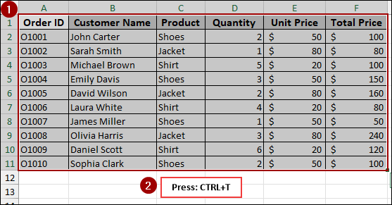
➤ Select your entire data range.
➤ Go to Insert > Table, or simply press Ctrl + T .
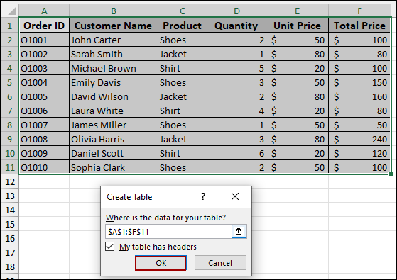
➤ In the Create Table dialog box, ensure the correct range is selected, and click OK.
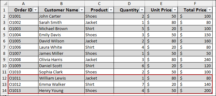
Your data range is now an Excel Table. Now, add the new rows of data directly below your existing table. Excel will automatically expand the table to include the new rows.
➤ Go to PivotTable Analyze > Data > Refresh and select Refresh.
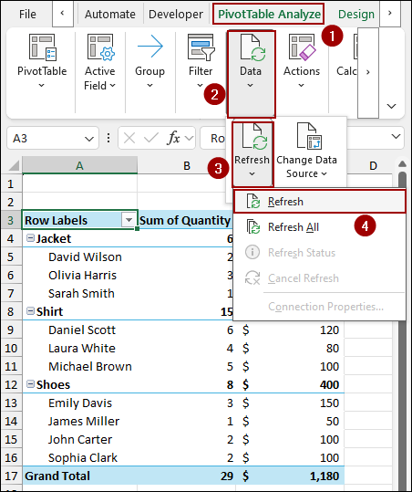
As a result, your Pivot Table will instantly update, including the new data you just added. This method is highly recommended as it automates the process of adding new rows.

Combining OFFSET and COUNTA Functions
For a more advanced solution, you can create a dynamic named range that automatically expands as you add new rows. Here, we will use the combination of OFFSET and COUNTA functions to create a dynamic named range. Thus, whenever new rows are included, they will automatically be added to the Pivot Table.
➤ Go to Formulas > Defined Names > Name Manager.
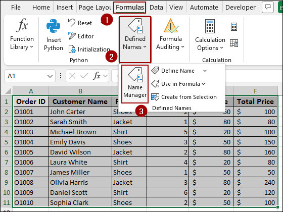
➤ In the Name Manager dialog box, click New.
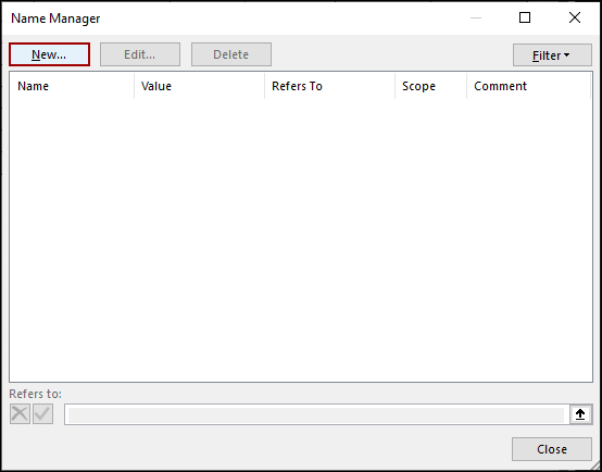
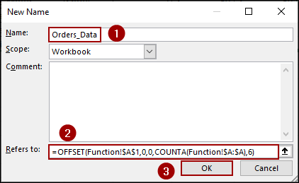
➤ In the New Name dialog box, you will create a name for your dynamic range (e.g., Orders_Data).
➤ In the Refers to field, enter the following formula.
=OFFSET(Function!$A$1,0,0,COUNTA(Function!$A:$A),6)
➤ Click OK to save the newly named range.
➧ Function!$A$1: It is the starting point of the data.
➧ 0,0: It means we are not moving from the starting row or column.
➧ COUNTA(Function!$A:$A): It counts the number of non-blank cells in column A, giving the number of rows in the dataset.
➧ 6: It is the number of columns in our data (A to F).
Now, create your Pivot Table from this named range.
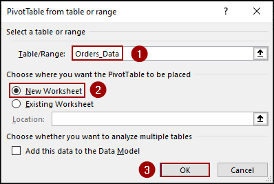
➤ Go to Insert > PivotTable.
➤ In the PivotTable from table or range dialog, type the name of your dynamic range (Orders_Data) and click OK.
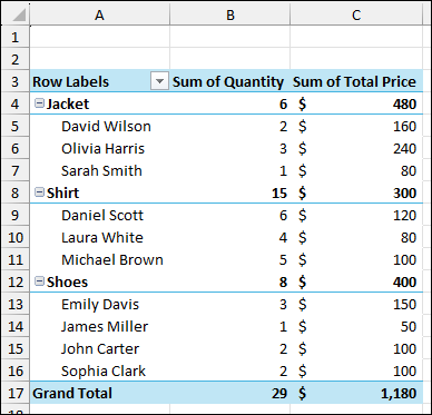
Thus, the Pivot Table will be created, connected to a dynamic range.
Now, let’s add some new rows of data in the source sheet.
➤ Go to PivotTable Analyze > Data > Refresh and select Refresh.

Finally, newly added rows are updated in the Pivot Table.

Frequently Asked Questions
Can I add new rows directly inside the Pivot Table?
No, you cannot type or insert rows directly into a Pivot Table. Always add rows in the source dataset and then refresh.
Why does my Pivot Table still not expand even though my data is in a Table?
If you added new rows, but they didn’t show up, make sure you clicked inside the Table when typing new data. Also, check if the Pivot Table’s source is still linked to the Table (sometimes it reverts to a fixed range).
My Pivot Table shows duplicate rows after adding data. How do I fix this?
Check the source dataset. If rows are truly duplicates, remove them before refreshing. If not, ensure you have arranged Pivot Table fields correctly.
Concluding Words
Above, we have explored various methods for adding rows to a Pivot Table in Excel. By using features like the Change Data Source tool, dynamic named ranges with OFFSET and COUNTA functions, or simply converting your data into an Excel table, you can ensure your analysis remains up-to-date. The most effective solution is to always use an Excel Table for your source data, as it automatically includes new entries. If you have any further questions, feel free to leave a comment below.