Pivot Tables in Excel are mostly used for data analysis and summarization. Sometimes, you may face an issue where your Pivot Table fails to recognize a date field, treating it as a standard number or text. This happens when the dates are not in the proper format. When Excel doesn’t recognize a date, it can’t group it by year, month, or day, which is one of the most powerful features of Pivot Tables. Instead, you will see a long list of individual dates or a strange sequence of numbers.
In this article, we will walk you through several methods to solve Pivot Table not recognising dates in Excel.
To solve Pivot Table not recognizing dates in Excel, here is one simple solution by converting to the proper date format.
➤ Select the dates and click on the Home tab.
➤ In the Number Format section, choose Date.
➤ Click OK and drag the Date field again to the Rows area in the Pivot Table Fields pane.
➤ Dates in the Pivot Table will be grouped, confirming that the Pivot Table is recognizing dates properly in Excel.
Converting to Proper Date Format
The most common reason a Pivot Table doesn’t recognize dates is that the dates are not formatted correctly. Even if the cells look like dates, Excel might be treating them as text or general numbers. The simplest solution is to convert the entire column to a date format.
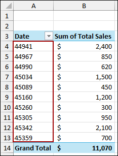
Let’s use a sample dataset with a “Date” column that is not being recognized by a Pivot Table. If we create a Pivot Table from this data, Excel will treat the “Date” column as a regular list of numbers instead of a date series.
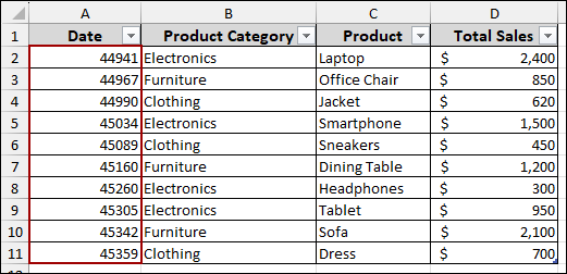
➤ Select your dataset.
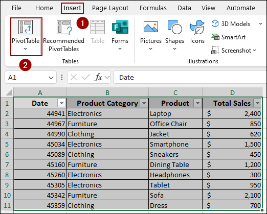
➤ Click Insert on the ribbon.
➤ In the Tables group, click PivotTable.
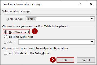
➤ In the PivotTable from table or range dialog box, select New Worksheet and click OK.
➤ In the PivotTable Fields pane, drag the Date field to the Rows area and the Total Sales field to the Values area.
As you can see, the dates are listed as five-digit numbers, which is how Excel stores dates internally when it doesn’t recognize them as a valid date format.
To fix this, we need to format the original data.
➤ Go back to your source data.
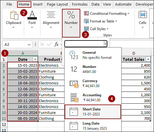
➤ Select the entire Date column.
➤ On the Home tab, in the Number group, click the dropdown menu.
➤ Select Short Date from the list.
This way, the values will be formatted as dates.
➤ Now, move to the Pivot Table sheet and right-click on any date in the Pivot Table.
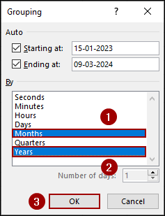
➤ Select Group from the context menu.

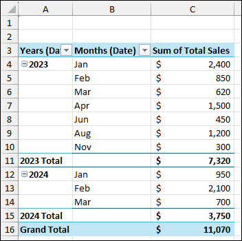
➤ In the Grouping dialog box, select Months and Years.
➤ Click OK.
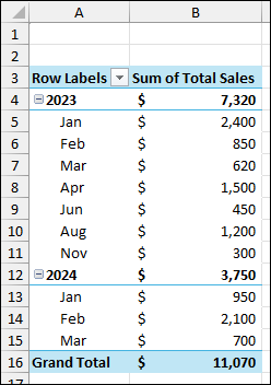
As a result, the Pivot Table will now display the date grouped by year and month, as it should. This way confirms that dates are recognized in the Pivot Table.

Utilizing Filter to Remove Errors and Text
Sometimes, a single text entry or an error value within your date column can prevent the entire column from being recognized as dates. These non-date values can be difficult to spot, but the filter feature can solve this issue.
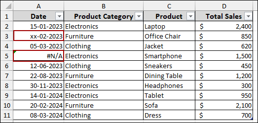
Consider a dataset with a couple of incorrect entries, such as text or an error value. If you create a Pivot Table with this data, it will not group the dates correctly because of these non-date entries. To fix this, we will use the filter on the source data.
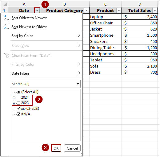
➤ Click on the dropdown arrow in the header of the Date column.
At the bottom of the filter list, you will see the incorrect entries, such as xx-02-2023 and #N/A. As we have to fix those incorrect entries manually, we will uncheck the correct date entries.
➤ Uncheck the boxes with correct date entries.
➤ Click OK.
Now, we will get the wrong entries shown in the table.
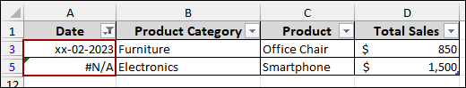
➤ Type the proper dates, removing the errors.

➤ Click the Filter icon from the Date column, checkmark Select All, and hit OK.
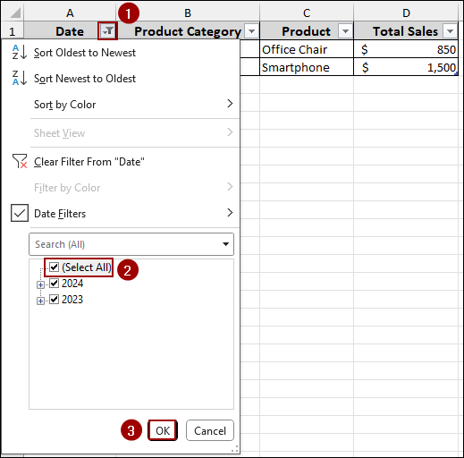
This way, we will get the dates correctly formatted removing the errors.

Finally, create the Pivot Table from the table, and you will see that the new Pivot Table will recognize dates properly.
Removing Extra Space from the Date Column in the Main Data Table
Another issue that can cause dates to be unrecognized is extra spaces before or after the date string. These extra spaces make Excel treat the entry as text rather than a date. While you can manually remove them, for a large dataset, a faster method is to use a simple copy-paste trick.
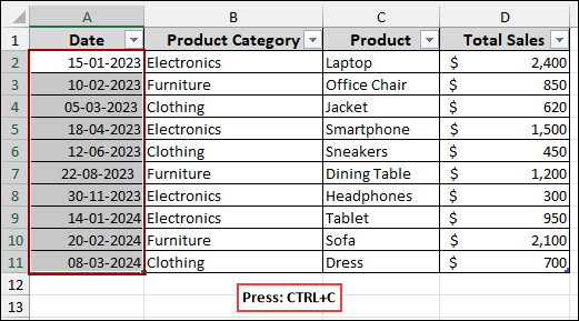
Consider a dataset where some date cells have extra spaces. Here, these dates look like dates, but they are preventing the Pivot Table from recognizing them.

If we create a Pivot Table from this data, the dates with spaces will not be grouped, as shown in the Pivot Table below.

To remove the extra spaces,
➤ Select the entire date column in your source data.
➤ Press Ctrl + C to copy the data.
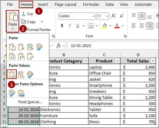
➤ Right-click, and from the Paste options, select Values.
This pastes the data without any hidden formatting or spaces.
➤ Now, remove the spaces from the table.

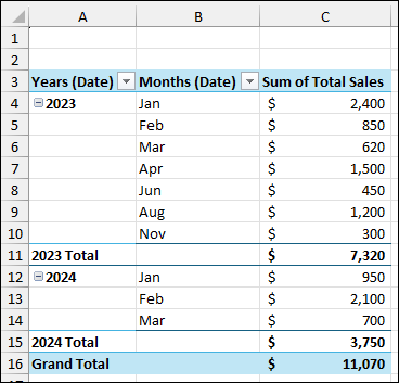
Finally, when we refresh the Pivot Table, all dates will be recognized and grouped correctly.
Frequently Asked Questions
How can regional date formats affect Pivot Table recognition?
Excel uses the system’s locale to recognize dates. Dates in formats like DD-MM-YYYY vs MM-DD-YYYY may not be recognized correctly. Convert them to a standard format compatible with your system.
Does copying data from another application cause this issue?
Yes, data copied from PDFs, web pages, or other applications often contain invisible characters or are stored as text. Cleaning and converting the data is necessary when you import from other sources.
Why does refreshing the Pivot Table not fix the issue?
Refreshing updates the Pivot Table, but it cannot convert text to dates. Conversion must happen in the source data.
Concluding Words
Above, we have explored several ways to solve Pivot Table not recognizing dates in Excel. By using the methods of formatting cells, filtering out errors, or removing extra spaces, you can resolve the problem easily. The most recommended approach is to ensure your source data is in the proper date format from the start. If you need assistance with similar Pivot Table adjustments, feel free to share them below.