When working with interactive Excel dashboards, invoices, or order forms, it’s common to have a drop-down list that controls what appears in another cell. For example, you might choose a product from a drop-down menu and have Excel automatically display its Sales, category, or stock status in another cell. This is called linking a cell value to a drop-down list, and it’s a powerful way to make your spreadsheets dynamic and user-friendly.
In this article, we’ll walk you through multiple effective methods to link a cell value with a drop-down list. These range from the classic VLOOKUP function to more modern techniques like FILTER function, ensuring compatibility with all Excel versions. Let’s get started.
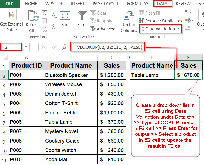
Steps to link a cell value with a drop down list in Excel:
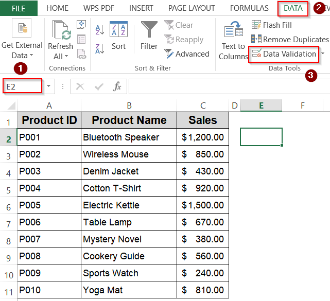
➤ Create a drop-down list for Product Name in cell E2 by selecting the cell >> Go to the Data tab >> Click on Data Validation.
➤ Under Allow, choose List and in the Source box, select B2:B11 >> Click OK.
➤ Select a product like Table Lamp from the list.
➤ In cell F2, type this formula:
=VLOOKUP(E2, B2:C11, 2, FALSE)
➤ Press Enter for output.
Using VLOOKUP Function for Retrieving Related Values from Drop-Down Selections
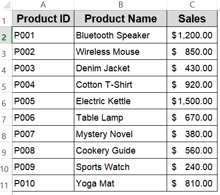
When you have a drop-down list in Excel and want a related value (like Sales, category, or stock level) to appear automatically based on the selection, the VLOOKUP function is a reliable and straightforward option. For example, suppose you have a dataset in cells B2:C11 containing Product ID, Product Name,and Sales figure. We’ll create a drop-down list for Product Name and link it so that selecting a product automatically shows related information in another cell. This method works best for neatly organized, vertical datasets where the lookup value is in the first column of the range.
This is the sample dataset we will be using:
Steps:
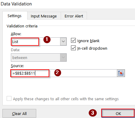
➤ Create a drop-down list for Product Name in cell E2 by selecting the cell >> Go to the Data tab >> Click on Data Validation.

➤ Under Allow, choose List.
➤ In the Source box, select B2:B11 >> Click OK.
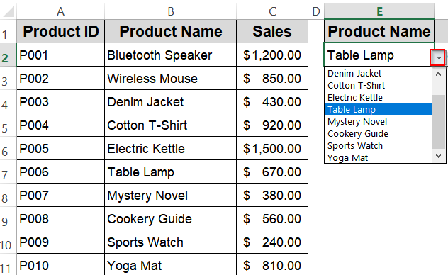
➤ Select a product like Table Lamp from the list.
➤ In cell F2, type this formula:
=VLOOKUP(E2, B2:C11, 2, FALSE)
Here, E2 is the drop-down cell with the product selection, B2:C11 is the table where column 1 contains product names and column 2 contains Sales figures, 2 specifies the return column, and FALSE ensures an exact match.
➤ Press Enter for output.
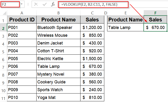
Now, whenever you select a product in E2, its Sales will instantly appear in F2.
Linking a Cell Using INDEX and MATCH Functions for Flexible Lookup
When you want to link a cell value based on a drop-down selection but your lookup column is not the first column in your dataset, the INDEX and MATCH combination is the perfect solution. For example, imagine you have a product list with columns for Product ID (A2:A11), Product Name (B2:B11), and Sales (C2:C11). Your drop-down menu in cell E2 lets you select a product name, and you want to automatically display its corresponding Sales in cell F2. INDEX and MATCH will look for the selected product in the product name column and return the matching Sales from the Sales column, no matter where those columns are placed.
Steps:
➤ Create a drop-down list for Product Name in cell E2 by selecting the cell >> Go to the Data tab >> Click on Data Validation.
➤ Under Allow, choose List and in the Source box, select B2:B11 >> Click OK.

➤ In cell F2, type this formula:
=INDEX(C2:C11, MATCH(E2, B2:B11, 0))
Here, C2:C11 is the range with the values you want to retrieve (e.g., Sales), E2 is the cell containing your drop-down selection, B2:B11 is the range where Excel looks for the selected product name and the 0 in MATCH ensures an exact match is found.
➤ Press Enter for output.
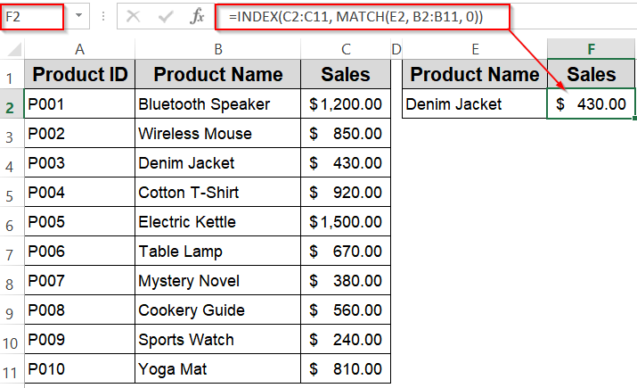
Now the corresponding Sales figure for the Product Name in E2 will display automatically.
Inserting the SUMIF Function to Calculate Values Based on a Drop-Down Selection
The SUMIF function is perfect when you want to connect a drop-down selection to a calculated numeric result, such as summing total sales or quantities related to the chosen item. Instead of returning a single value, SUMIF adds up all values that meet the criteria specified by the drop-down choice, making it useful for summarizing data dynamically.
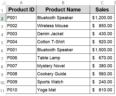
For example, suppose your dataset contains product names in B2:B11 and their corresponding sales figures in C2:C11. By selecting a product in the drop-down at E2, you can use SUMIF to total all sales for that product automatically.
This is the modified dataset we will be using:
Steps:
➤ Create a drop-down list in cell E2 as in the previous methods.
➤ In cell F2, type this formula:
=SUMIF(B2:B11, E2, C2:C11)
Replace C2:C11 with the actual range containing the numeric values you want to sum (in this example, it represents sales figures).
➤ Press Enter for output.
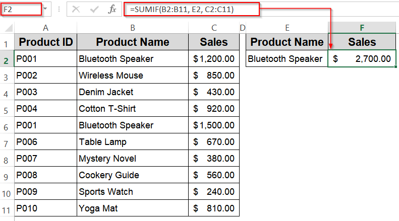
Now the formula sums all values in the numeric range where the product name in B2:B11 matches the selected product in E2 such as Bluetooth Speaker.
Applying the INDIRECT Function with Named Ranges for Dynamic Cell References
The INDIRECT function converts text into a valid cell or range reference, making it perfect for situations where your drop-down selection determines which named range or cell Excel should use. Instead of a fixed lookup, INDIRECT allows your formula to dynamically adapt based on the drop-down choice.
For example, if each product has its own named range representing its stock status such as Bluetooth_Speaker, Wireless_Mouse, and so forth, you can use INDIRECT function to fetch the correct stock information automatically when a product is selected from the drop-down list.
Steps:
➤ Replace all spaces in the Product Name column with an underscore.
➤ Create named ranges for each product’s Sales figure cell. For instance, select the cell C2 for the Sales figure of the Bluetooth Speaker, and name this range Bluetooth_Speaker (replace spaces with underscores).
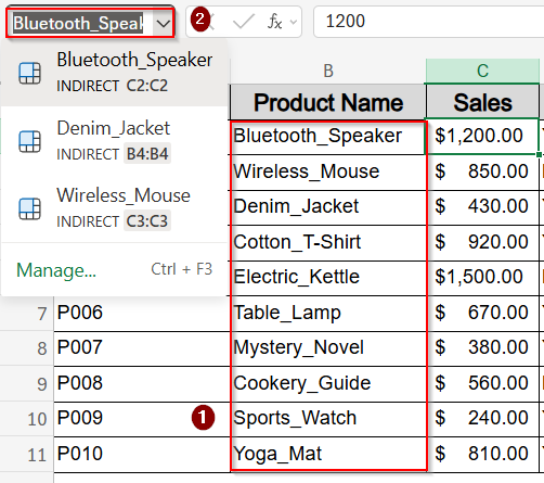
➤ Set up a drop-down list in E2 containing product names formatted exactly like the named ranges (use underscores instead of spaces).
➤ In cell F2, type the formula:
=INDIRECT(E2)
➤ Press Enter for output.
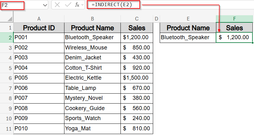
Now when you select a product in E2, INDIRECT converts that text into the corresponding named range and returns the Sales value automatically.
Using the FILTER Function to Retrieve Multiple Related Values
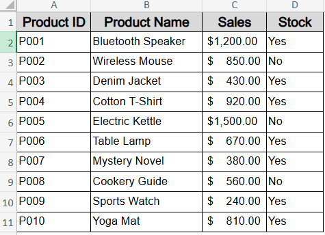
The FILTER function, available in Excel 365 and Excel 2021, is designed to return multiple matching results dynamically. This makes it perfect when you want to display several related values based on a single drop-down selection. For example, you can retrieve both the Sales and Stock status for a selected product without writing separate formulas for each.
This is the dataset we will be using:
Steps:
➤ Create the drop-down list in cell F2 as done in previous methods.
➤ In cell G2, enter the formula:
=FILTER(C2:D11, B2:B11=F2)
This formula filters the range C2:D11 (Sales and Stock columns) to return rows where the product name in B2:B11 matches the selected item in F2.
➤ Press Enter and the formula will spill automatically.
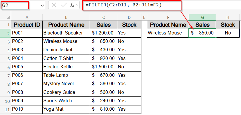
The result displays both the Sales and Stock status for the selected product side by side.
Frequently Asked Questions
Can I link more than one value to a single drop-down selection?
Yes. You can link multiple outputs to a single drop-down selection by either using the FILTER function to return several results at once, or placing separate formulas in adjacent cells to retrieve different corresponding values.
Do I need to sort my dataset for these methods to work?
No. Sorting isn’t required for these methods. VLOOKUP and INDEX with MATCH functions both work with unsorted lists when you set the match type to FALSE (or 0), ensuring they search for exact matches rather than approximate ones.
Which method works best in all Excel versions?
For maximum compatibility, use VLOOKUP or INDEX with MATCH functions . Both are supported in all Excel versions. However, FILTER function is available only in Excel 365 and Excel 2021, making it version-dependent for modern dynamic array functions.
Can I use these methods to pull data from another sheet or workbook?
Yes. Simply reference the other sheet or workbook in your formulas. For example, with VLOOKUP or INDEX with MATCH, include the sheet name before the range, or link an external file using full file path syntax.
Wrapping Up
In this tutorial, we explored five effective ways to link a cell value with an Excel drop-down list using functions like VLOOKUP, INDEX and MATCH, INDIRECT, FILTER, and SUMIF. Each method serves different needs starting from retrieving a single value, to displaying multiple linked results, to dynamically referencing ranges. With these techniques, you can make your spreadsheets more interactive, automate lookups, and reduce errors caused by manual entry. Feel free to download the practice file and share your feedback.