
Working with large Excel spreadsheets can be visually tiresome. Highlighting the active row can make it easier to track data while navigating through rows. This feature is good during data entry, reviewing datasets, or while presenting data live. In this process, when we click on a cell, the related row automatically gets highlighted with the pre-defined colour.
To highlight the active row in Excel, follow these steps:
➤Press Alt + F11 to open the VBA Editor.
➤Insert a new module and paste a VBA code that highlights the active row.
➤Close the editor and run the macro or use Worksheet events for automatic highlighting.
In this article, you will learn how to highlight the active row in Excel using a conditional formatting, VBA-based and a mix of conditional formatting and VBA scripting method.
Using Conditional Formatting and VBA to Highlight Active Row in Excel
We can use Conditional Formatting and VBA to Highlight Active Row in Excel when we want to highlight the currently selected row automatically. This is good when we work with large datasets like task trackers, sales logs, or attendance sheets. This method works without defining the name and complex code.
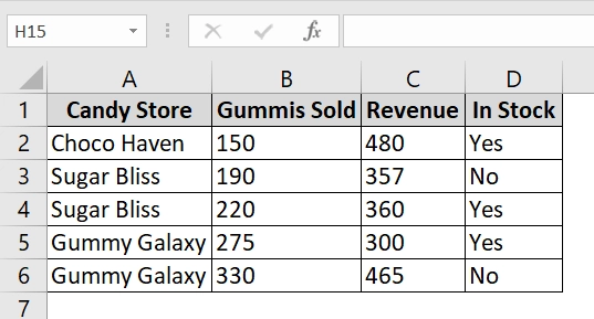
We have a dataset that contains Candy Store Status. We will highlight the entire row of active cells dynamically using this method.
Steps:
➤ Open your Excel Worksheet. We have taken a table containing Candy Store Name in Column A, Gummies Sold in Column B, Revenue in column C, and Stock Product in Column D.
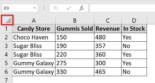
➤ Select the whole worksheet by clicking on the top left box.
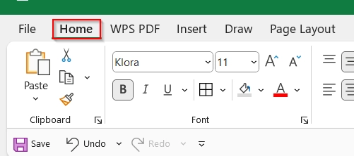
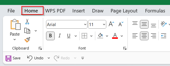
➤ Go to the home tab from the Ribbon.
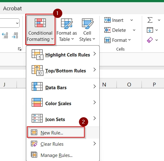
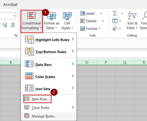
➤ Click on Conditional Formatting > New Rule.
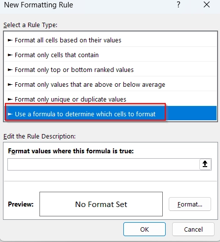
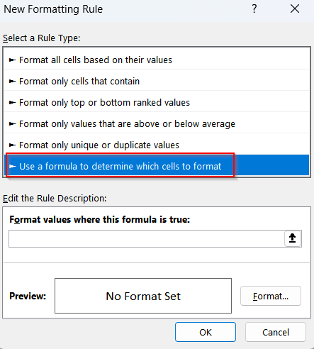
➤ Choose: “Use a formula to determine which cells to format”
➤ In the formula box, paste the following formula, and click on the format.
=row()=cell("row")
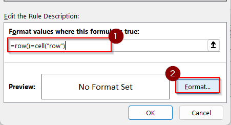
➤ Then, Click to the Fill tab → choose a highlight color (e.g., light yellow). Click OK twice to apply the rule.

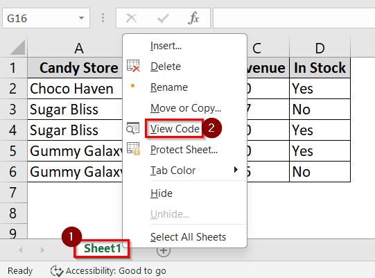
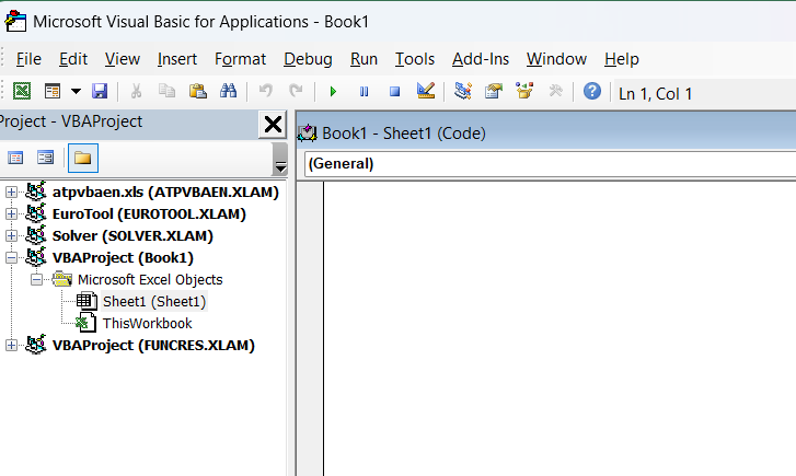
➤ Right-click the sheet tab (e.g.,sheet1 ”) → select View Code.
➤ An interface like this will be opened.
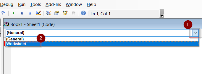
➤ Click the dropdown on the code window. Then, select “Worksheet”.
➤ Paste the following VBA code between the first and second line:
Target.Calculate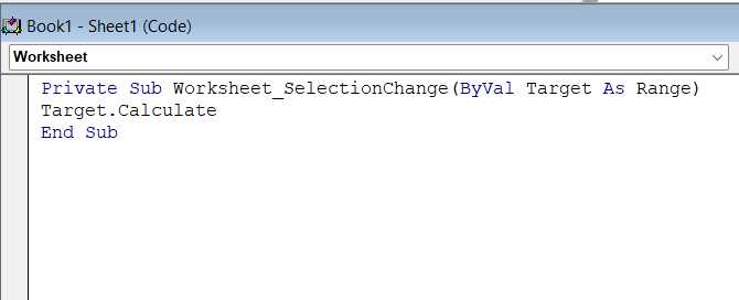
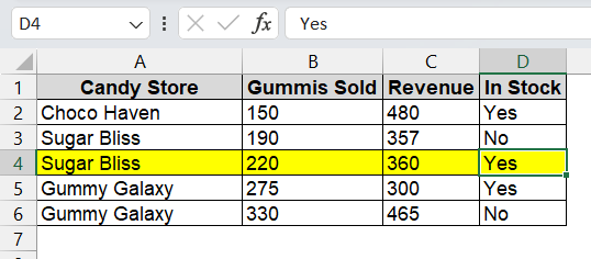
➤ Now return to the worksheet and click on various cells throughout the sheet. The entire row of the selected cell will now be highlighted in the color you set. If I click on cell D4, the Row 4 gets highlighted.
Applying VBA Macro to Highlight Active Row in Excel
VBA Code is used to dynamically highlight the row containing the active cell. This technique is good when we work with wide or long datasets. We use this method to apply across any Excel worksheet.
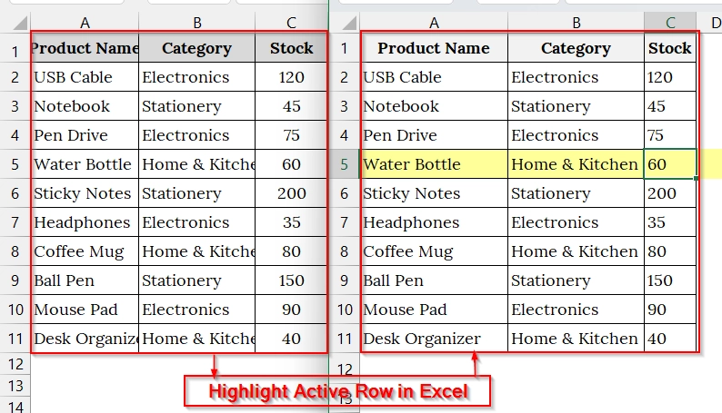
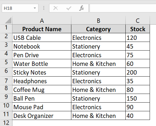
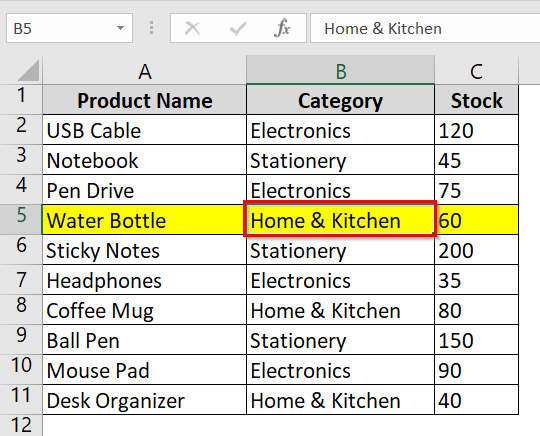
We have a table that relates to the product Name, Category, and Stock of a store. We will highlight the active row to avoid editing the wrong product using the VBA method.
Steps:
➤ Open your Excel file. We have taken a dataset that contains Product Name in Column A, Category in Column C, and Stock in Column C.
➤ Press Alt + F11 , or use Fn + Alt + F11 to open the VBA Editor.
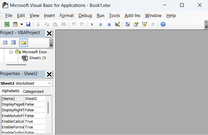
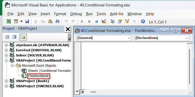
➤ In the VBA editor, double click on “ThisWorkbook” in the left-hand Project pane
➤ Paste the following code in the “ThisWorkbook” code window. This code listens for selection changes and formats the active row with a light yellow fill (RGB(255, 255, 153).
Private Sub Workbook_SheetSelectionChange(ByVal Sh As Object, ByVal Target As Range)
    Static oldRow As Range
    Application.ScreenUpdating = False
    Cells.FormatConditions.Delete
    Target.EntireRow.FormatConditions.Add Type:=xlExpression, Formula1:="=ROW()=ROW(INDIRECT(""RC"",FALSE))"
    Target.EntireRow.FormatConditions(1).Interior.Color = RGB(255, 255, 153)
    Application.ScreenUpdating = True
End Sub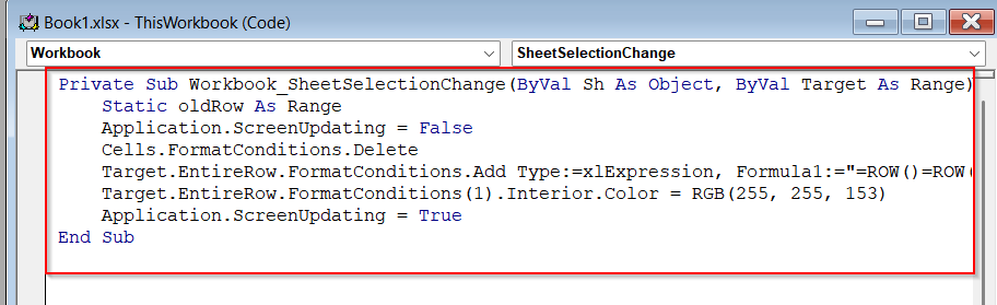
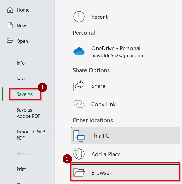
➤ Go to the File tab from the Ribbon.
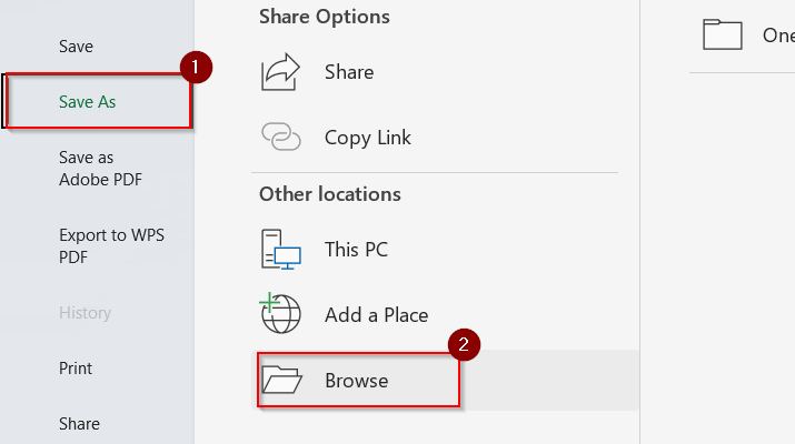
➤ Click on Save as and Select Browser.
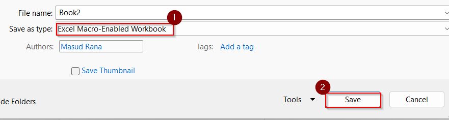
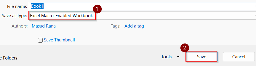
➤ Now, in the save as type, choose: “Excel Macro-Enabled Workbook” from the dropdown list in. Then, click Save.
➤ Close the VBA editor and return to Excel. Test it by clicking on different cells
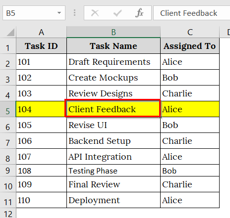
The active row will highlight automatically as you move between cells. Here, we have selected the B5 cell and the whole Row 5 got highlighted.
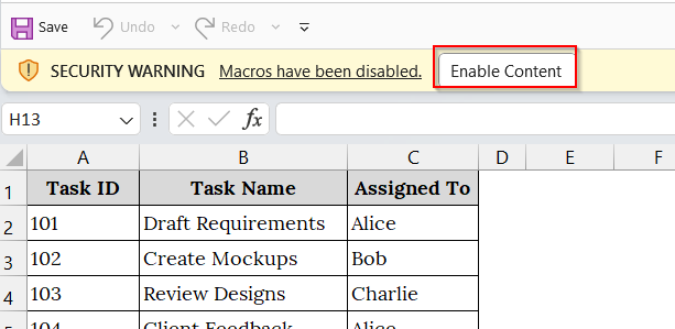
➤ When you open the file next time, Excel will ask to enable macros – click “Enable Content” to activate this feature.
Note:
➥Excel Online and Excel for Web do not support VBA, so this method will not work there.
➥You can change the highlight color by modifying the RGB(…) values in the code.
➥This highlight is temporary and resets every time you switch sheets or close the workbook unless re-enabled.
Use of Conditional Formatting & VBA to Highlight Active Row in Excel
We use this method when we want to highlight the currently selected row automatically using a mix of conditional formatting and VBA script. This is best when we work with large datasets like task trackers, sales logs, or attendance sheets where following the active row visually is important.
We have a dataset that contains a project task tracker. We will locate the row (task) which is actively editing or reviewing using this method.
Steps:
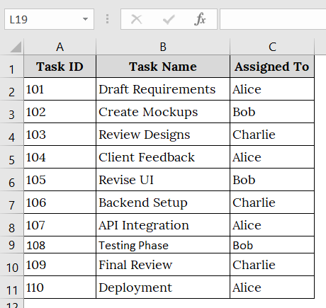
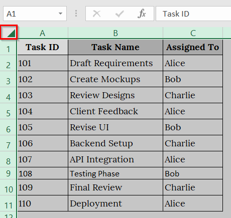
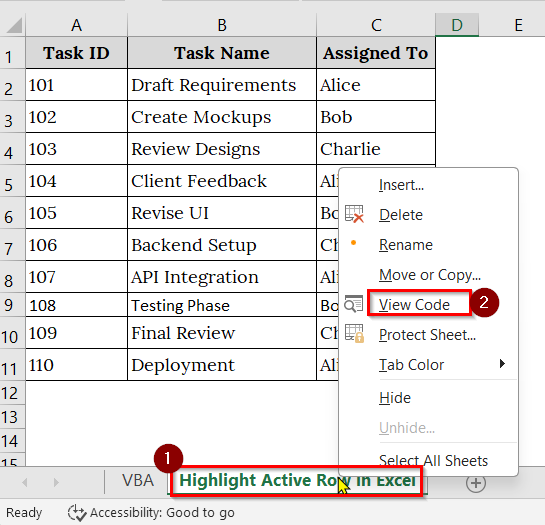
➤ Open your Excel Worksheet. Here, we have taken a table containing Task ID in Column A, Task Name in Column B, and Assigned Name in Column C.
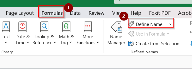
➤ Go to the Formulas tab in the ribbon and click on Define Name.
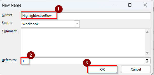
➤ In the Name box, enter: HighlightActiveRow, in the Refers to box, enter: = and Click OK to save.
➤ Click the small triangle icon at the top-left corner (above row 1 and left of column A) to select all cells.
➤ Go to the home tab from the Ribbon.
➤ Click on Conditional Formatting > New Rule.
➤ Choose: “Use a formula to determine which cells to format”
➤ In the formula box, paste the following formula, and click on the format.
=ROW(A1)=HighlightActiveRow
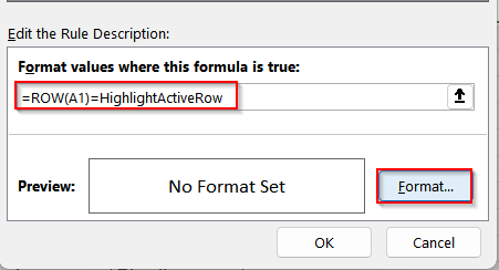
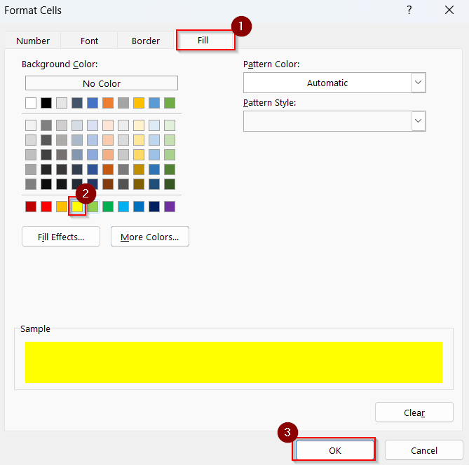
➤ Then, Click to the Fill tab → choose a highlight color (e.g., light yellow). Click OK twice to apply the rule.
➤ Right-click the sheet tab (e.g.,sheet 3 Named as Highlight Active Row in Excel ”) → select View Code.
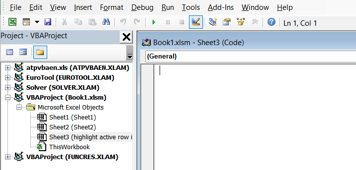
➤ An interface like this will be opened.
➤ Paste the following VBA code:
Private Sub Worksheet_SelectionChange(ByVal Target As Range)
    With ThisWorkbook.Names("HighlightActiveRow")
        .Name = "HighlightActiveRow"
        .RefersToR1C1 = "=" & ActiveCell.Row
    End With
End Sub 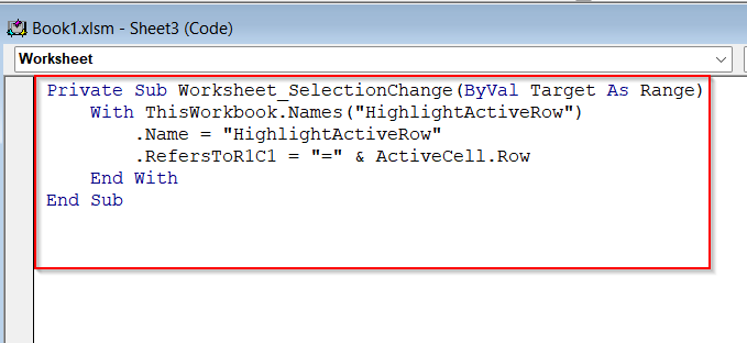
➤ From the File Tab, Click on Save as and choose Browser.
➤ Choose format Excel Macro-Enabled Workbook (*.xlsm)
➤ Click on various cells throughout the sheet. The entire row of the selected cell will now be highlighted in the color you set. For example, we have selected the entire B5 cells.
Note:
➥This does not override other formatting rules already applied to cells.
➥The method works per worksheet. Repeat steps for each worksheet where needed.
Ensure macros are enabled when reopening the file or this feature won’t function.
Frequently Asked Questions
Can I highlight the active row without VBA?
Yes, but it requires helper cells and formulas with conditional formatting. However, it’s not truly “dynamic” like the VBA method.
Does this work on Excel for Mac?
Yes, but Mac users must enable macros and use the VBA editor accordingly.
Will it highlight multiple selected rows?
The VBA method focuses on a single active cell. For multiple selections, you’d need a more advanced macro.
Does this work in Google Sheets?
No, this method is exclusive to Microsoft Excel. Google Sheets does not support VBA.
Concluding Words
The best method to highlight the active row in Excel is by using VBA. It allows dynamic row highlighting as you move through your spreadsheet while increasing focus and productivity. Once set up, it updates automatically and works seamlessly during navigation. Conditional Formatting in Excel is best to highlight a specific row when macros are a bit restricted.