With Excel’s conditional formatting feature, you can highlight cells that contain any text from a predefined list. It’s often used for tasks like flagging specific products, identifying key customers, categorizing feedback, or tracking project statuses.
Functions like COUNTIF, SEARCH, MATCH, SUMPRODUCT, etc., allow you to highlight cells based on an exact or partial match from a list. The simplest way for all Excel versions is to use the COUNTIF function to set formatting rules.
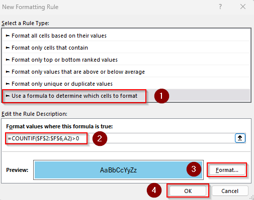
➤ Select the range (A2:A10) to highlight and go to the Home tab >> Conditional Formatting drop-down >> New Rule >> Use a Formula to Determine Which Cells to Format.
➤ In the Format Values Where This Formula Is True field, insert the following formula:
=COUNTIF($F$2:$F$6,A2)>0
➤ Replace $F$2:$F$6 with the range containing the list and A2 with the first cell of the range you want to highlight. Use the Format button to set formatting styles and press Ok.
This article covers all the ways of highlighting cells based on a list using the COUNTIF, SEARCH, ISNUMBER, MATCH, and SUMPRODUCT functions.
Highlight Cells Matching a List Using the COUNTIF Function
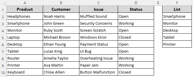
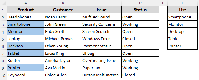
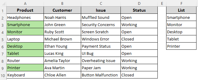
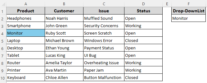
Our sample dataset for customer issues has columns for Product, Customer names, Issue description, and Status. In Column F, we have a list of 5 products based on which we’ll apply the highlighting rules.
With the COUNTIF function, we can look for exact matches from a list. Here’s how:
Format a Single Column
➤ Select the column range you want to format (without the header). For our dataset, we chose the A2:A10 range.
➤ Open the Home tab, click on the Conditional Formatting drop-down, and select the New Rule option from the menu.

➤ When Excel opens the New Formatting Rule dialog box, select Use a Formula to Determine Which Cells to Format.
➤ In the Format Values Where This Formula Is True field, enter the following formula:
=COUNTIF($F$2:$F$6,A2)>0

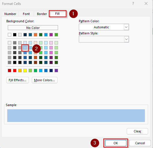
➤ Press the Format button and select your preferred formatting styles using the Number, Font, Border, and Fill tabs. Click Ok once you’re done.
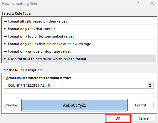
➤ Check the Preview box to see what the formatted text will look like. Finally, press Ok.
➤ Here’s the final output:
Format the Entire Row
➤ Click and drag to select your entire data range (A2:D10) and go to the Home tab >> Conditional Formatting drop-down >> New Rule >> Use a Formula to Determine Which Cells to Format.
➤ In the formula box, type the following formula:
=COUNTIF($F$2:$F$6,$A2)>0
➤ Replace the cell references as needed. Set the formatting rules using the Format option and click Ok when done.

➤ Click Ok to close the New Formatting Rule dialog box and see the final result.

Format Matching Texts Using the ISNUMBER and MATCH Functions
To find exact matches from a list, combine the ISNUMBER and MATCH functions as shown below:
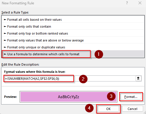
➤ Select the range (A2:A10) to highlight and go to the Home tab >> Conditional Formatting drop-down >> New Rule >> Use a Formula to Determine Which Cells to Format.
➤ In the formula field, insert the following formula:
=ISNUMBER(MATCH(A2,$F$2:$F$6,0))
➤ Here, A2 is the first cell of the column containing the matching texts and $F$2:$F$6 is the list. Change these values to match your dataset.
➤ Click on Format and choose highlighting options. Press Ok when done.
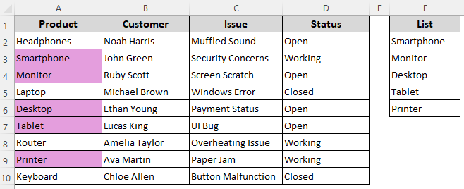
➤ Close the dialog box by clicking Ok so that Excel displays the highlighted cells.
Applying Conditional Formatting Formula with COUNT and SEARCH Functions
As the SEARCH function only finds the first match, we’ll combine it with COUNT to create a conditional formatting formula that finds all the matches from a list. Below are the details:
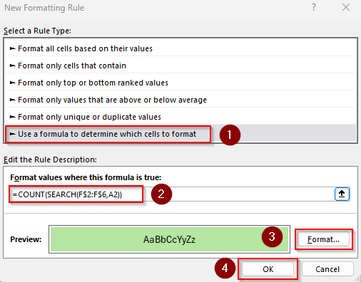
➤ Select your data range (A2:A10) and go to the Home tab >> Conditional Formatting drop-down >> New Rule >> Use a Formula to Determine Which Cells to Format.
➤ Insert the following formula in the designated field for formula:
=COUNT(SEARCH(F$2:F$6,A2))
➤ Press Format to choose the colors, fonts, etc., to highlight the cells. Click Ok when you’re done.
➤ Click Ok to see the highlighted cells:
Highlight Cells with When Value Partially Matches a List
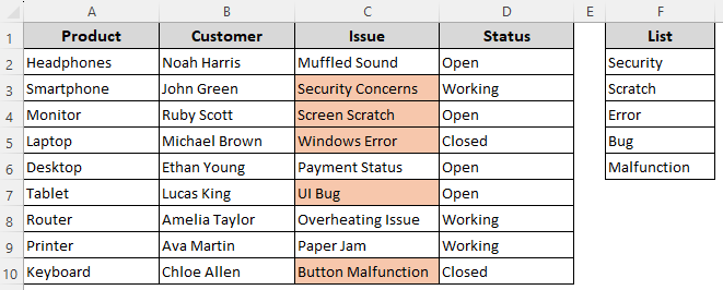
When you don’t know the entire text string to match a list, you can use the COUNTIF and SUMPRODUCT functions with wildcards. Here, we have a list containing parts of a text string like outage Error, Security, Bug, etc. We’ll look for these values in Column C. Let’s get to the steps:
➤ Select the range to highlight (C2:C10) and open the Home tab >> Conditional Formatting drop-down >> New Rule >> Use a Formula to Determine Which Cells to Format.
➤ In the formula box, insert the following formula:
=SUMPRODUCT(COUNTIF($C2, "*" & $F$2:$F$6 & "*"))>0
➤ $C2 is the first cell of the column containing the texts we want to match and $F$2:$F$6 is the list. Replace the values according to your dataset.
➤ Set the formatting rules and press Ok.

➤ Click Ok again to see the result:
Highlight Partial Matches with the SEARCH and SUMPRODUCT Functions
Similar to COUNTIF, the SEARCH function can also be combined with SUMPRODUCT to format partial matches. Here’s how:
➤ Click and drag to highlight your data range (C2:C10) and go to the Home tab >> Conditional Formatting drop-down >> New Rule >> Use a Formula to Determine Which Cells to Format.
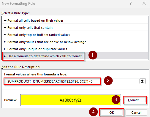
➤ Paste the following formula in the formula field:
=SUMPRODUCT(--ISNUMBER(SEARCH($F$2:$F$6, $C2)))>0
➤ Change the cell references as required.
➤ Select the formatting styles and press Ok.
➤ Click Ok to close the dialog box and get the output.

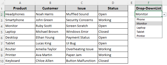
Format Cells Containing Text from a Drop-Down List
To create a drop-down list, select the cell(s) where you want the drop-down (F2). Go to the Data tab >> Data Validation. In the Allow box, choose List. Proceed to the Source box and type the items you want to list, separated by commas (e.g., Laptop, Tablet, Phone). The drop-down list should look like this:
Now, to highlight cells matching a drop-down list, follow the steps given below:
➤ Select the range you want to highlight (A2:A10) and click on the Home tab >> Conditional Formatting drop-down >> New Rule >> Use a Formula to Determine Which Cells to Format.
➤ In the formula box, type any of the following formulas:
Formula for Exact Match
=$A2=$F$2
➤ In cell $F$2, we have the drop-down and our selected value from the list. $A2 is the first cell of our selected range. Replace these values according to your dataset.
➤ Choose the formatting rules and press Ok.

➤ Click Ok to check the final output.
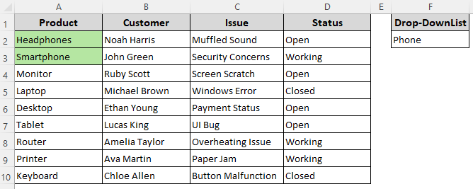
Formula for Partial Match
=ISNUMBER(SEARCH($F$2,$A2))
➤ Change the cell references as required to match your dataset.
➤ Set the formatting rules and click Ok.

➤ Press Ok again to see the formatted cells.
Frequently Asked Questions
How to highlight cells in Excel based on a list in another sheet?
First, select the range to highlight (B2:B10), and go to the Home tab >> Conditional Formatting drop-down >> New Rule >> Use a Formula to Determine Which Cells to Format. In the formula box, enter:
=COUNTIF(Sheet2!$A$2:$A$5,B2)>0
This formula highlights cells in Column B if they match any value from Sheet2!A2:A5. Replace the values as needed, set formatting rules, and press Ok twice.
How do I highlight cells in Excel that are not in a list?
Select the range to highlight (B2:B10) and click on the Home tab >> Conditional Formatting drop-down >> New Rule >> Use a Formula to Determine Which Cells to Format. In the formula field, type:
=COUNTIF($F$2:$F$6,$B2)=0
It highlights all cells in Column B that do not appear in the list F2:F6. Set formatting rules and click Ok twice.
How do you highlight cells that have the same value in Excel?
Select your range (A2:D10) and go to the Home tab >> Conditional Formatting >> Highlight Cells Rules >> Duplicate Values. Choose your preferred formatting styles and press Ok twice.
Concluding Words
Choose a suitable formula based on the type of your list and the outcome you want. Lock the first cell of your range with a dollar sign ($) to highlight the entire row. If your list has items that don’t match any of the values in your selected range, the formulas won’t return an error. However, you must make sure the list doesn’t contain blanks.