Highlighting the highest value in Excel can help you quickly spot top-performing figures whether you’re tracking sales, scores, or any numerical data. Instead of scanning manually, Excel offers a smart way to apply Conditional Formatting that highlights the max value automatically, even as the data updates.
In this article, you’ll learn how to highlight the highest number in Excel using built-in formatting tools, custom formulas, and row-by-row methods. Each technique ensures your spreadsheet stays dynamic and easy to read.
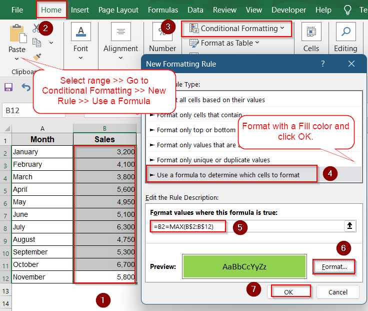
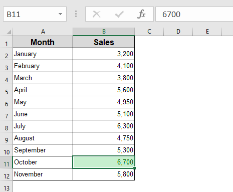
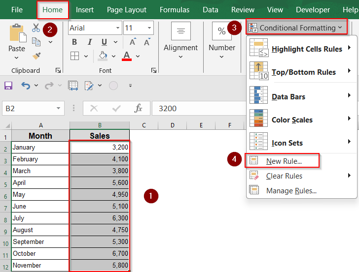
➤ Select the full data range (e.g., B2:B12).
➤ Go to Home >> Conditional Formatting >> New Rule.
➤ Choose “Use a formula to determine which cells to format”.
➤ Use this formula: =B2=MAX(B$2:B$12)
➤ Click Format >> Select a fill color and press OK.
Highlight Highest Value in a Column (Top 1 Rule)
This built-in Excel rule quickly highlights the highest number in a column. It’s a great no-formula solution when you want to automatically spot the single top value or even the top N values at a glance.
Steps:
➤ Select the range with numbers (e.g., B2:B12).
➤ Go to Home >> Conditional Formatting >> Top/Bottom Rules >> Top 10 Items…
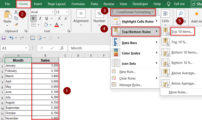
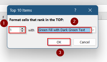
➤ In the dialog box, change 10 to 1.
➤ Choose a format style (like a bold fill color).
➤ Click OK.
Note:
If you enter N instead of 1, the top N highest values will be highlighted.
This highlights the single highest value in your selected range. It adjusts automatically if the values change.
Use MAX Function to Track the Highest Cell Value
For more control, use the MAX function inside a custom rule to highlight the highest value. This method is ideal when you need dynamic updates as data changes, and it works well for datasets not limited to a single column.
Steps:
➤ Select the full data range (e.g., B2:B12).
➤ Go to Home >> Conditional Formatting >> New Rule.

➤ Choose “Use a formula to determine which cells to format”.
➤ Use this formula:
=B2=MAX(B$2:B$12)
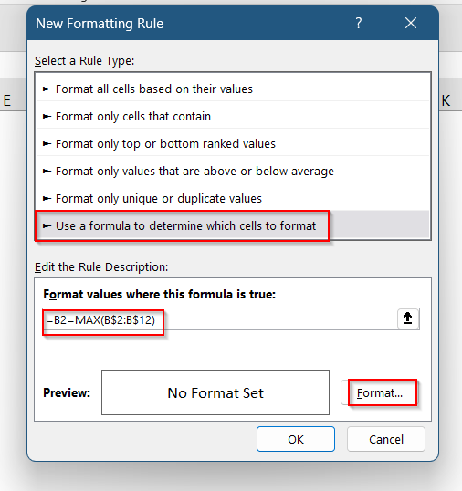
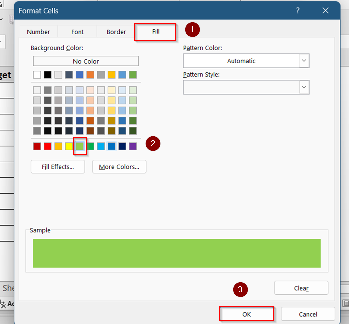
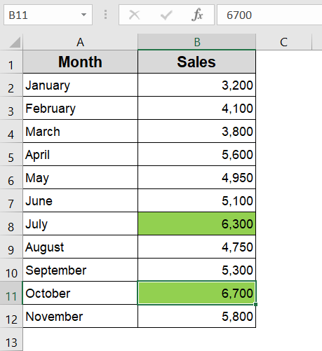
➤ Click Format, select a fill color (e.g., green), and press OK.
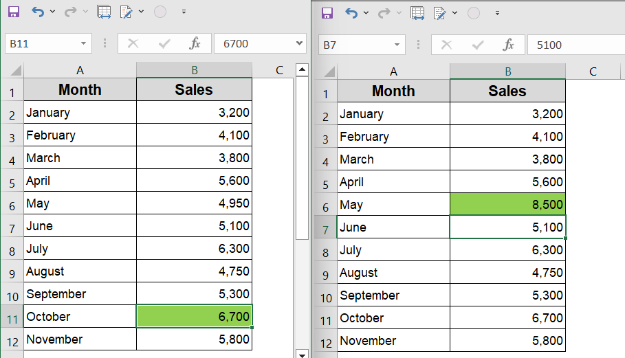
Now, only the cell with the maximum value will be highlighted. It updates automatically when the data changes.
Apply LARGE Function to Mark Top N Entries
The LARGE function lets you highlight not just the maximum but any top N values. This approach gives you flexibility to track the top 3, top 5, or any number of highest values dynamically using Conditional Formatting.
Steps:
➤ Select the range (e.g., B2:B12).
➤ Go to Home >> Conditional Formatting >> New Rule.

➤ Choose “Use a formula to determine which cells to format”.
➤ Enter this formula (to highlight top 3 values):
=B2>=LARGE($B$2:$B$12,3)
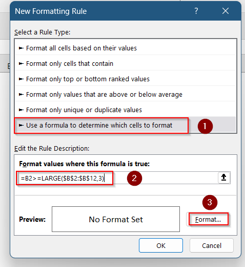
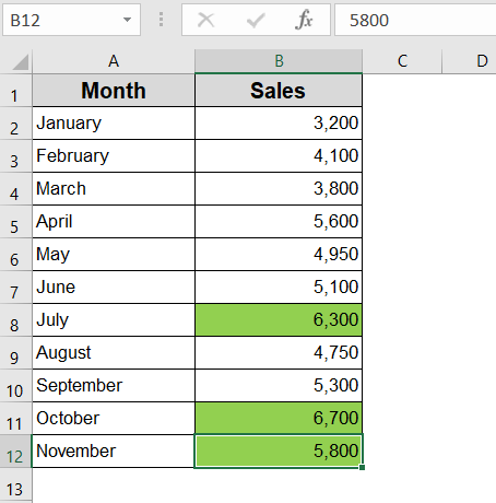
➤ Click Format, select your desired Fill color, and click OK.

This method highlights all values that are greater than or equal to the third-largest value in the range.
Visualize Highest Numbers with Data Bars
Data Bars provide a built-in way to visualize relative values directly inside cells. With just a few clicks, you can compare all entries visually, making it easy to spot higher or lower values without needing to apply formulas or rules.
Steps:
➤ Select your numeric range (e.g., B2:B12).
➤ Go to Home tab >> click Conditional Formatting.
➤ Choose Data Bars >> select a Gradient Fill or Solid Fill style.
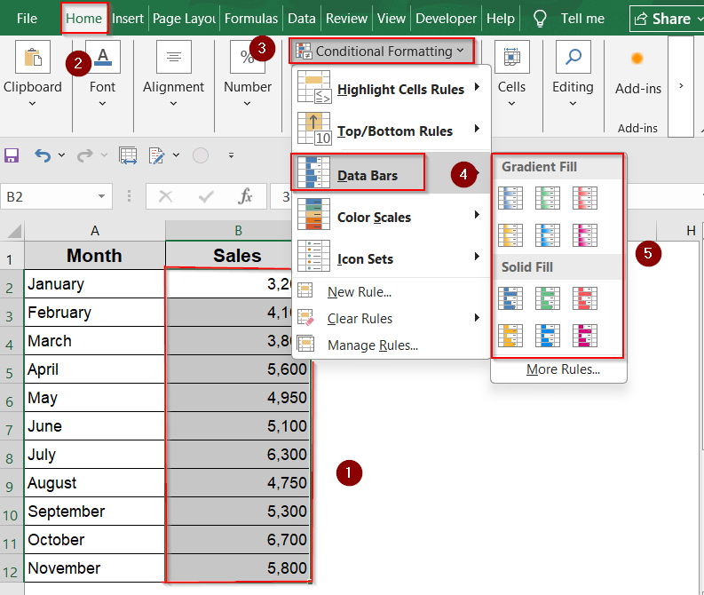
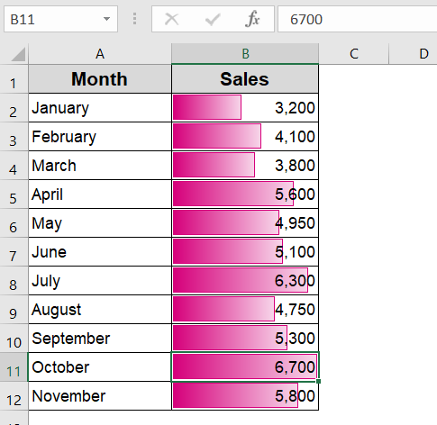
This will insert bars within the cells, with longer bars representing higher values.
Create Conditional Ranking for Smart Formatting
This method uses a formula that combines RANK.EQ with a condition to highlight top values only if they exceed a defined threshold. It’s ideal when you want to spotlight high performers without cluttering your spreadsheet with unnecessary highlights.
Steps:
➤ Select the range (e.g., B2:B12)
➤ Go to Home >> Conditional Formatting >> New Rule.
➤ Choose “Use a formula to determine which cells to format”.
➤ Enter the formula:
=AND(RANK.EQ(B2, $B$2:$B$12)<=3, B2>6000)

➤ Click Format, select your desired Fill color, and click OK.

This rule will highlight the maximum value only if it exceeds 6000.
Frequently Asked Questions
How do I highlight the top value across an entire Excel sheet?
Use the formula =A1=MAX($A$1:$Z$100) in conditional formatting and adjust the range to fit your dataset.
Can I highlight the top 3 values instead of just the top 1?
Yes, use the built-in “Top 10 Items” rule and change the number to 3. Excel will highlight the top 3 numbers automatically.
Will the highlighting update if I change the data?
Absolutely. All these methods are dynamic and will automatically re-evaluate the top values whenever the data changes.
Can I apply conditional formatting to both rows and columns at once?
Yes, but you’ll need to apply separate conditional formatting rules with different formulas for rows and columns.
How do I remove the formatting?
Go to Home > Conditional Formatting > Clear Rules and choose either “Clear Rules from Selected Cells” or “Entire Sheet”.
Wrapping Up
In this tutorial, we explored how to highlight the highest value in Excel using built-in rules and custom formulas. Whether you’re focusing on columns, rows, or full tables, Excel makes it easy to visually spotlight the most important figures. Feel free to download the practice file and share your feedback.