Highlighting selected cells in Microsoft Excel is a necessary technique in order to improve data usability, highlight important information, and facilitate data analysis. Excel has several methods for highlighting cells- whether you want to highlight particular values, distinguish data sets, or call attention to particular entries. These techniques include conditional formatting based on formulas or rules as well as manual formatting.
Steps to highlight selected cells in Excel using Conditional Formatting:
➤ Select the cell range or column you want to apply the formatting to.
➤ Go to the Home tab > Click Conditional Formatting > Choose Highlight Cells Rules.
➤ Select a condition (e.g., “Greater Than”, “Less Than”, “Equal To”) according to your desired results.
➤ Input your value and choose a preferred formatting colour option.
➤ Click OK.
We have discussed multiple ways to highlight selected cells in Excel in this article. From simple manual formatting to dynamic, rule-based techniques like Conditional Formatting and VBA macros- you will find them all in this guide with detailed steps.
Highlight Selected Cells with Manual Formatting
If you have certain cells selected, manual formatting can be the easiest method for you to do this. This method will be the best for one-time or visually-driven highlights that don’t need to change automatically.
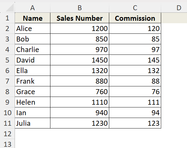
Suppose, this is our dataset where we want to highlight the cells under the column C.
Follow these steps to complete the highlighting manually:
➤ Select the cells you want to highlight. We are selecting from cell C2 to cell C11 because we want to highlight the values in Column C.
➤ Go to the Home tab on the ribbon.
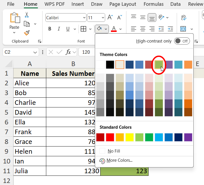
➤ Click the Fill Color icon (paint bucket symbol) in the Font group.
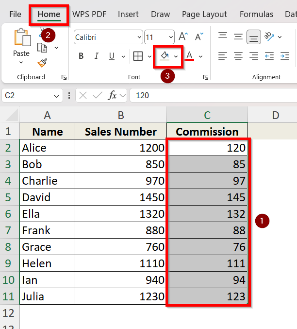
➤ Choose a color from the palette. We are choosing this Olive Green (accent 3) colour as the highlight.
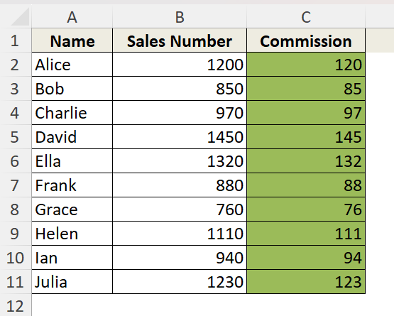
Here we have our selected cells highlighted perfectly.
Apply Conditional Formatting Based on Cell Value to Highlight Selected Cells
This method is perfect for when you want Excel to automatically highlight cells that meet specific numerical or text-based conditions. You can apply the formatting only in your desired cell ranges.
For example, we want to highlight the cells that are only greater than 100 in column C. Follow these steps to apply the conditional formatting and get desired results:
➤ Select the cells or range you want to apply the formatting to. We are selecting column C as this is where we want to apply the formatting in.
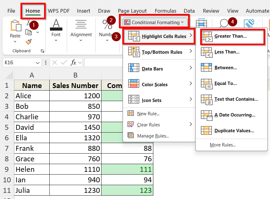
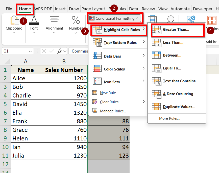
➤ Go to the Home tab > Click Conditional Formatting > Choose Highlight Cells Rules.
➤ Select a condition (e.g., “Greater Than”, “Less Than”, “Equal To”). Since we want to highlight cells Greater than 100, we will choose the Greater Than option.
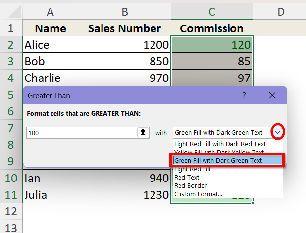
➤ In the pop-up box, type in the value you want the cells to be greater than. We are typing in 100 in this box.
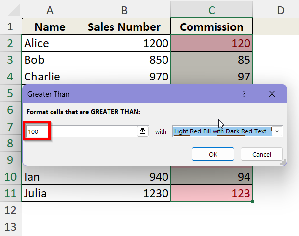
➤ Choose the formatting style from the drop-down box beside. We are selecting the Green Fill with Dark Green Text option. Click OK.
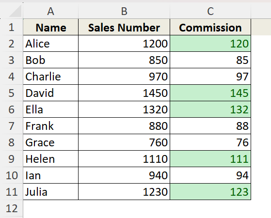
➤ Now, we will have our desired cells highlighted in column C which are all greater than 100.
Use a Custom Formula in Conditional Formatting to Highlight Selected Cells
Using a formula is ideal for complex rules that aren’t covered by standard conditional formatting options.
Suppose, we want to highlight the entire rows where sales exceed 1000 in the dataset. We will use a custom formula for this by going through these steps one by one:
➤ Select the range of cells, which in this case, is the entire table.
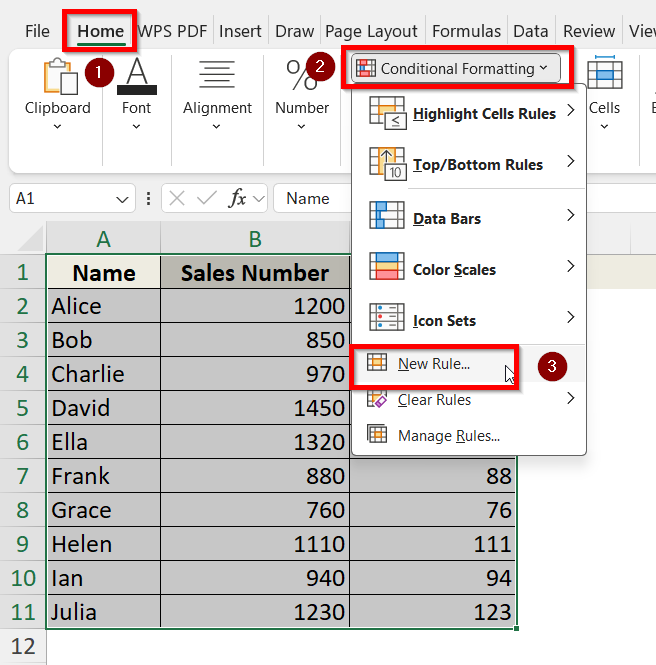
➤ Go to Home tab > click Conditional Formatting > select New Rule.
➤ In the New Formatting Rule dialog, choose Use a formula to determine which cells to format.
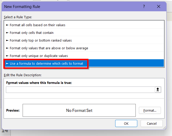
➤ Enter this formula in the formula box:
=$B2>1000
Here, this formula returns TRUE for rows where the sales number is greater than 1000. $B2 locks the column B (Sales Number) but allows the row to adjust as Excel checks each row.
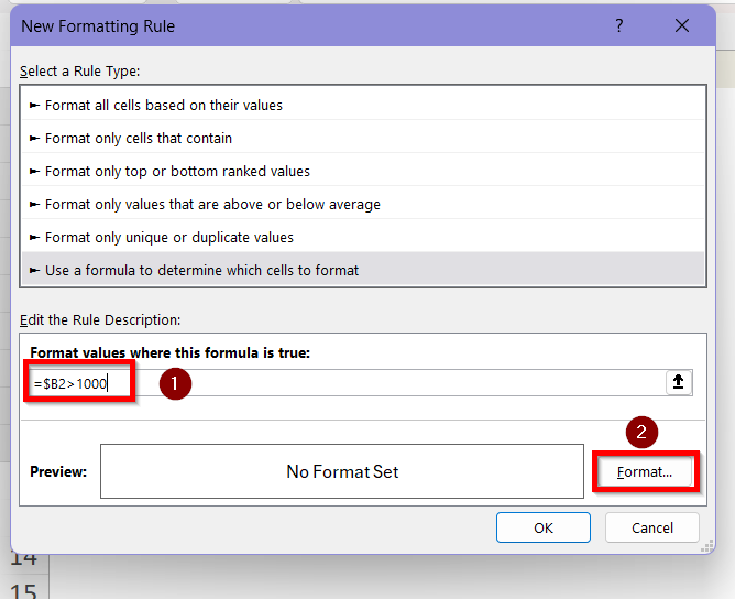
➤ Click Format.
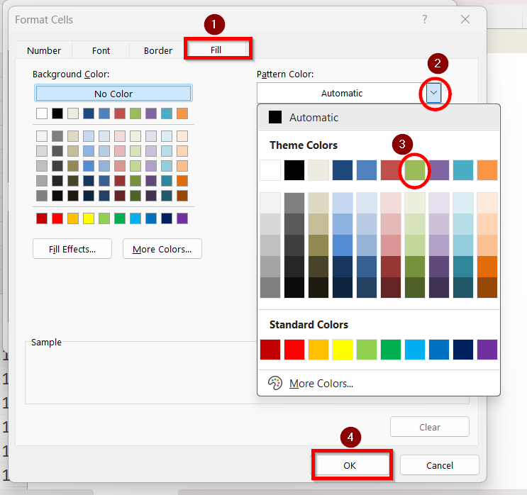
➤ In the Format Cells box, click on Fill and then select your desired color for the highlighted cell from the color pallete. We are choosing this Olive Green (accent 3) colour as the highlight. Click OK.
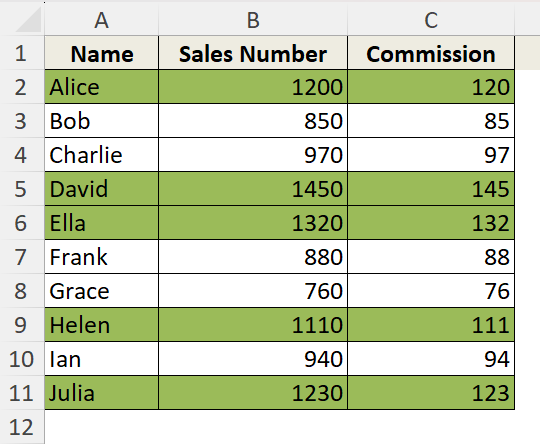
➤ Now, we have the rows highlighted where the sales exceed 1000.
Insert VBA Macro to Highlight Selected Cells
This method is used for automating custom cell highlighting based on complex or repeated tasks.
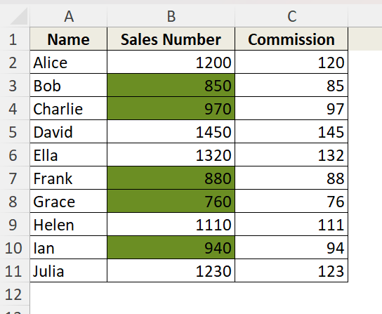
Suppose, we want to highlight the cells where sales number is lower than 1000 now. Here is a detailed guide on how you can use the VBA Macro to highlight those selected cells:
➤ Open your Excel Workbook and select column B as we want to highlight the cells which are less than 1000 here.
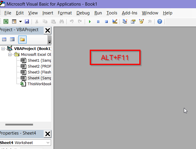
➤ Press Alt + F11 to open the Visual Basic Editor window.
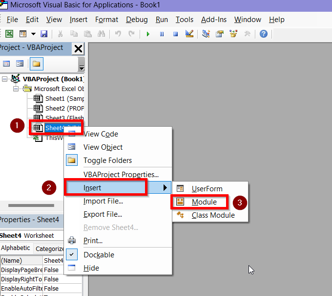
➤ Right click on the worksheet containing your data then go to Insert > Module.
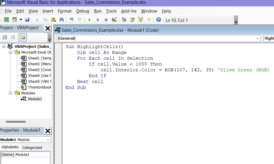
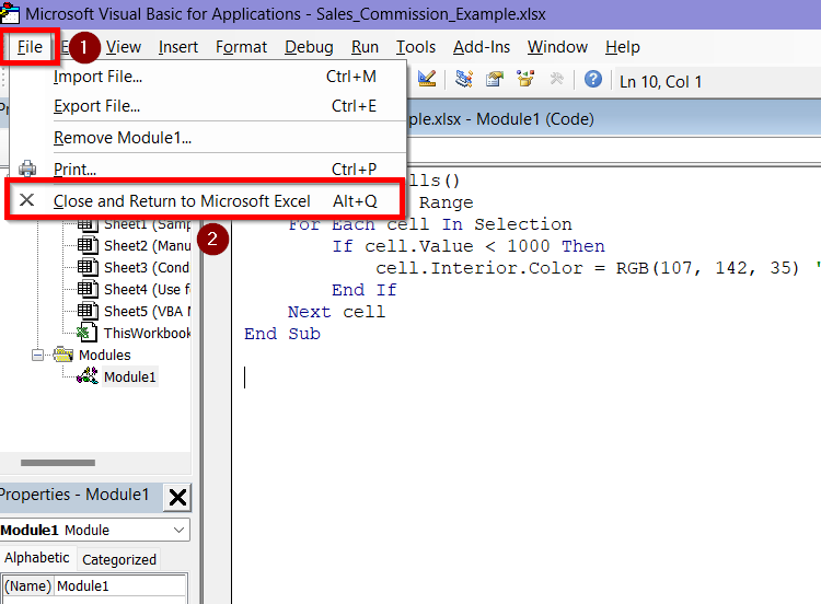
➤ In the new module, copy and paste the following code.
Sub HighlightCells()
    Dim cell As Range
    For Each cell In Selection
        If cell.Value < 1000 Then
            cell.Interior.Color = RGB(107, 142, 35)'Olive Green (RGB)
        End If
    Next cell
End Sub
➤ The code will look like this in the module:
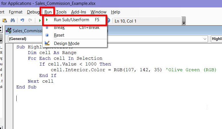
➤ Click on Run tab and select Run Sub/UserForm.
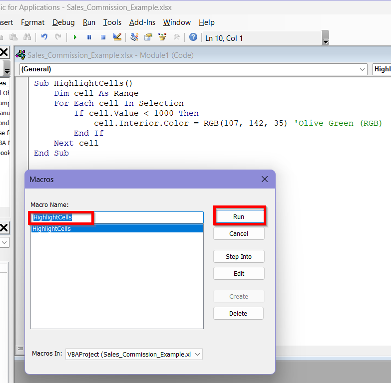
➤ In the Macros box, select the Macro Name as HighlightCells and then click Run.
➤ Go to the File tab and select Close and Return to Microsoft Excel.
➤ Back in the worksheet, we can now see the cells less than 1000 are highlighted in column B.
Frequently Asked Questions
What’s The Difference Between Manual Highlighting and Conditional Formatting?
Manual highlighting is a static and time consuming method. You need to choose the cells individually which you want to highlight and then apply color in those cells.
On the other hand, conditional formatting is a dynamic method because it changes automatically based on values, rules, or formulas you set, without selecting the cells individually.
Is It Possible to Highlight Only Cells Containing Formulas?
Yes, you can highlight only the cells that contain formulas by using custom formula method in Conditional Formatting. Use the formula =ISFORMULA(A1) in conditional formatting New Rule segment.
Will Conditional Formatting Update Automatically if My Data Changes?
Yes, Conditional Formatting recalculates and reapplies the conditions in the selected cells after you change the data. As long as the rules remain the same, the new data will automatically be highlighted according to your condition.
Which Highlighting Methods Are The Best for Large Datasets?
Both VBA macros and Conditional Formatting are the best options to apply on large datasets. Manual highlighting should be avoided in these cases.
Wrapping Up
Manual highlighting is best suited for straightforward, static jobs while conditional formatting offers automation and flexibility based on predetermined rules or conditions. Formula-based highlighting enables row or column level logic easily. VBA enables personalized, repeatable automation which is particularly helpful in complicated or large datasets.
The type of data you have and how interactive or scalable you want your formatting to be will determine which approach is best for you. Hope you can choose the method best suited for you and present your data in a clear, presentable manner.