

Pulling data based on criteria means extracting specific data from one sheet/tab onto another sheet or tab. This process involves using formulas that follow certain rules. Some formulas return multiple results, while others give just one. This is super handy when dealing with large datasets and focusing on specific data.
In this article, I’ll show you how to pull data from another tab with step-by-step examples using functions like QUERY, FILTER, VLOOKUP, and more. With these functions, you will be able to perform actions such as list greater values, find low-stock items, show customer comments, extract tasks, spot duplicates, and create targeted reports.
Let’s get started!
Before we dive deeper, first, you have to create at least two sheets within the same Google Sheet. You can click the “+” icon on the bottom left side of the Google Sheet to create a new sheet. After that, follow the steps below:
➤ Now you have two spreadsheets inside one Google Sheet. To move some specific data from “Sheet1” to “Sheet2” without copying and pasting, go to “Sheet2” first
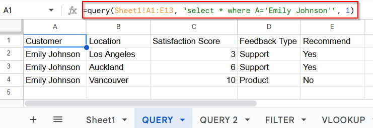
➤ Now apply this “Query” function in the A1 cell. The function is: “ =query(Sheet1!A1:E13, “select * where A=’Emily Johnson'”, 1) “
➤ After applying the function, just press Enter on the keyboard and your data will be extracted from “Sheet1” to “Sheet2
Apply QUERY Function to Pull Data From Another Sheet Based on Criteria
I’ll show you a simple example using practical images to pull data from the range A1:E13 in Sheet1 and extract it into Sheet2 (I named it Query. You can use any sheet or tab.) In this example, the formula will only return the rows where the value in Column A is Emily Johnson.
Steps:
➤ Open Your Google Sheet and Create Another Sheet in the same file.

➤ Head over to Sheet2, double click on A1 cell.
➤ Now copy and paste the query function below.
=query(Sheet1!A1:E13, “select * where A=’Emily Johnson'”, 1)
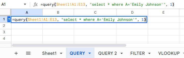
➤ Next, just press Enter.
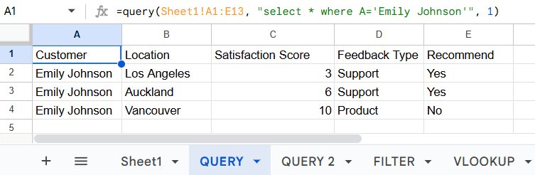
➤ Sheet1!A1:E13 refers to the range of rows and columns from which we want to pull the data.
➤ select * where A='Emily Johnson' means it will extract all rows where Column A contains Emily Johnson into Sheet2.
So, based on your dataset, you might need to adjust the function to fit your needs.
Another Application with the QUERY Function
This is another application of the QUERY function that I’m going to show you. It works the same way as the previous one. The only difference is that you can use this function to pull specific data based on a greater-than condition.
Steps:
➤ Create a New Sheet / tab (or apply it to your current sheet)
➤ Just like before, go to the new Sheet >> Cell A1 (or any cell). I’ve used a new sheet, as you can see, named Query 2.
➤ Write down the following formula in your output cell:
=query(Sheet1!A1:E13, “select * where A=’Emily Johnson’ and C>5”, 1)
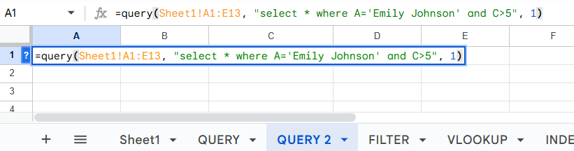
➤ Then press Enter.
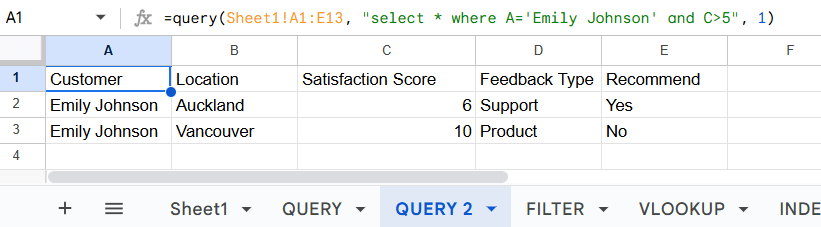
Inserting FILTER Function
With the FILTER function, you can easily pull data from one sheet to another based on specific criteria. This method extracts rows from one sheet and places them on another sheet that meets the defined requirements. It also updates automatically whenever you make changes to the original data in Sheet1.
Steps:
➤ Create a new sheet, or move on to any other sheet within the Google Sheets.
➤ Next, go to your selected sheet, where you want to extract your data using the Filter function.
➤ Go to A1 cell or any cell of that sheet and apply the following function:
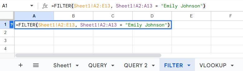
➤ Hit Enter
➤ And you’re all done
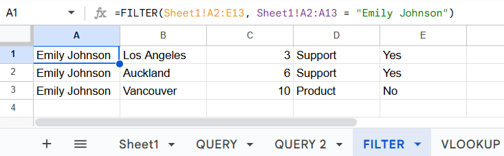
➤ Sheet1!A2:A13 = 'Emily Johnson': This part means that only the rows where Column A contains Emily Johnson will be extracted.
Now, based on your specific needs, you might change the function.
Pull Data From Another Tab Based on Criteria Using VLOOKUP Function
VLOOKUP function isn’t the best option for pulling multiple data from one sheet to another. However, if you only need to pull a specific or single piece of data from another sheet or tab, this method can be useful. I will use the same example of “Emily Johnson” in here as well.
Steps:
➤ As usual, keep your main sheet in the Google Sheet and create another sheet in the Google Sheet
➤ Then go to your new sheet that you just created, double click on any cell to apply the VLOOKUP formula. I’m using the B6 cell to keep things easy for you to understand. You can actually apply this formula in any cell.
➤ And apply the following function
=VLOOKUP(“Emily Johnson”, Sheet1!A2:E13, 2, FALSE)
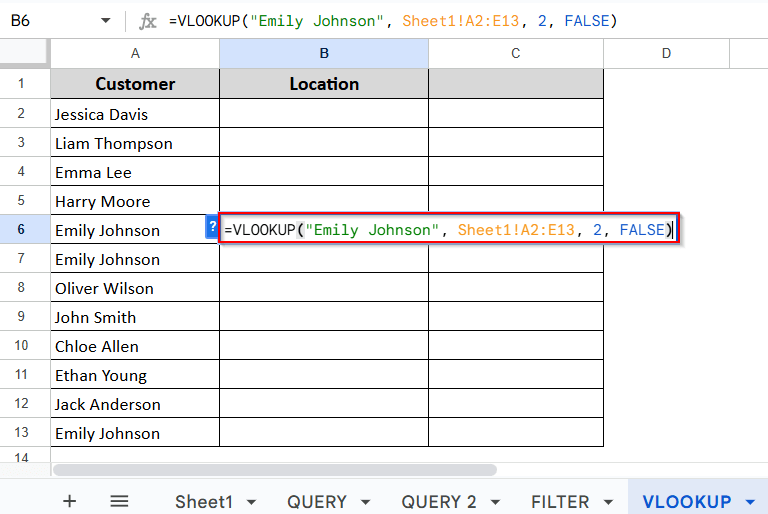
➤ Press Enter.
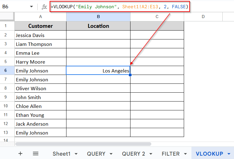
First, remember that VLOOKUP only works vertically. It looks for a value in the first column of the selected range and then pulls data from another column in the same row based on criteria. In our case, it found “Emily Johnson” in the first column and returned the value from a column we specified.
But that still doesn’t fully explain why “Los Angeles,” right? Here's why: after selecting the range Sheet1!A2:E13, I used 2, FALSE in the formula.
➤ Here, 2 means we are pulling the value from the second column of the selected range.
➤ So when it found Emily Johnson in Column A (the first column), it looked to Column B (the second column) of the same row, which contains Los Angeles. That’s why only Los Angeles appeared.
Now, if I change the formula to this:
=VLOOKUP(“Emily Johnson”, Sheet1!A2:E13, 3, FALSE)
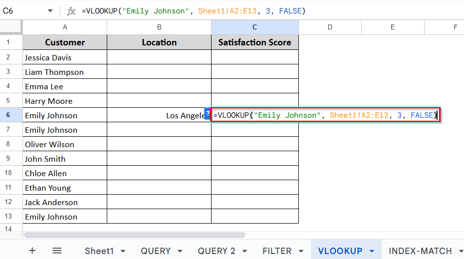
We are pulling the value from Column 3 instead. That would return the value from Column C in the same row as “Emily Johnson.” And again, to keep things consistent, I’m using the C6 cell. You can apply this formula in any cell.
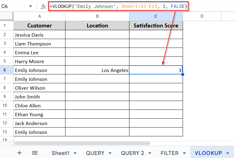
If you check the dataset I’m using, you’ll see that for the first Emily Johnson the value in Column C is 3, which is the satisfaction score. So now, 3 would be pulled instead of Los Angeles.
One last thing, if you’re wondering what FALSE means, it simply tells Google Sheets to find an exact match for Emily Johnson.
Combine INDEX and MATCH Functions to Pull Data
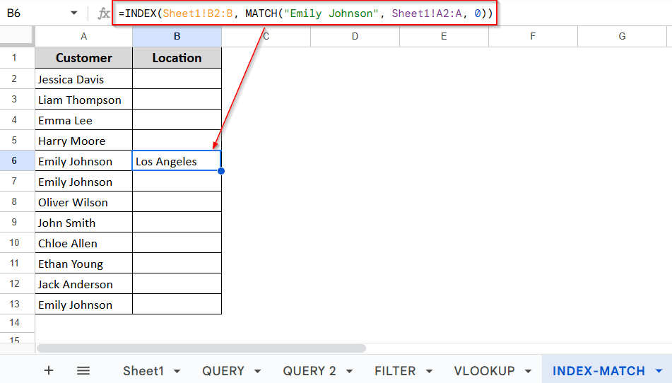
VLOOKUP function and INDEX-MATCH formula basically do the same thing. Both are useful for pulling specific data from another sheet. But neither is ideal if you’re trying to pull multiple rows of data at once. But when you just need to fetch a single piece of data like I did with VLOOKUP, INDEX and MATCH can be really handy.
The main advantage of INDEX and MATCH is that your data doesn’t have to be arranged in a specific order that was required for applying VLOOKUP function.
Steps:
➤ In your new sheet, go to any cell where you want to pull the data. I’m using the B6 cell.
➤ Use the following formula:
=INDEX(Sheet1!B2:B, MATCH(“Emily Johnson”, Sheet1!A2:A, 0))
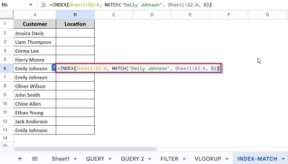
➤ Hit Enter.
Using ARRAYFORMULA & IF Functions for Pulling Multiple Matches
The combination of ARRAYFORMULA and IF functions work in the same way as the QUERY and FILTER functions. But there is a slight difference in how the data is pulled, which you will see in the images below.
Steps:
➤ In your new sheet, navigate to A1 cell or any cell
➤ Apply this formula
=ARRAYFORMULA(IF(Sheet1!A2:A13 = “Emily Johnson”, Sheet1!A2:E13, “”))
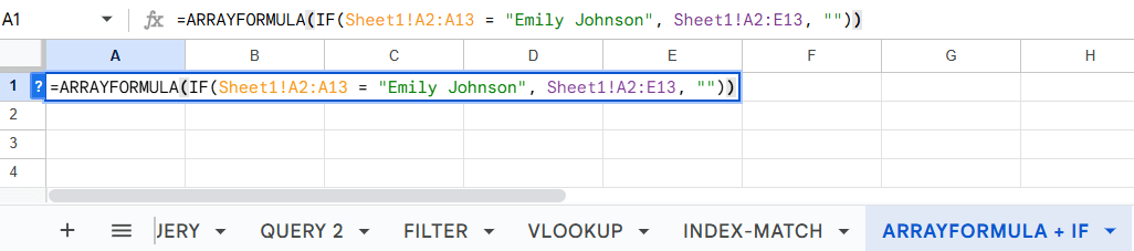
➤ Press Enter.
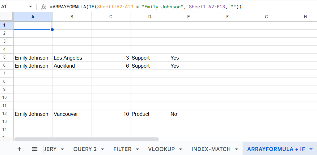
As you can see, the data extracted from Sheet1 is displayed in the same layout as it was in Sheet1. Not arranged in a clean, structured way. This is the main difference between ARRAYFORMULA-IF formula and the QUERY or FILTER functions.
Practice Resources
Get our practice workbook or necessary files that we have worked with to prepare this article.
Pull Data from Another Tab Based on Criteria in Google Sheets [Make a Copy]
Frequently Asked Questions
How do I pull a value from another tab in Google Sheets?
➤ Type “=” in target cell
➤ Click the source tab and the specific cell
➤ Press Enter, and the data appears.
How do I combine data from two Google Sheets?
➤ Open the sheet you want to pull data from and the sheet you want to add data into.
➤ Copy the full URL of the source sheet and note the tab name (Sheet1) and cell range (e.g., A1:E13).
➤ In the destination sheet, type:
=IMPORTRANGE(“URL”, “TabName!Range”)
➤ Example: =IMPORTRANGE(“https://docs.google.com/…”, “Sheet1!A1:E13”)
➤ Click Allow access, and all your data will appear in the new sheet.
Concluding Words
We’re at the end of this article. I’ve covered six methods with clear explanations on how to pull data from another tab based on specific criteria. Functions like Query, Filter, and ARRAYFORMULA + IF are designed for pulling multiple pieces of data at once from another tab. On the other hand, VLOOKUP and INDEX + MATCH are best for extracting a single value.
Now that you’ve learned all the methods for pulling data, you can use whichever one best suits your needs.