Combining the IMPORTRANGE and FILTER functions lets you pull and display data from another Google Sheet based on specific conditions. But when you need to apply multiple criteria, things get trickier. Google Sheets doesn’t offer native support for complex filters across files, so you’ll need a few smart formulas to make it work.
In this article, we’ll show four effective methods to filter data from an external file using more than one condition. Whether you’re managing reports, dashboards, or synced sheets, these techniques will help you get precise, live results.
Steps to filter data across Google Sheets using multiple IMPORTRANGE calls with the FILTER function:
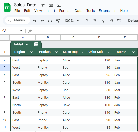
➤ Use the source dataset in the Sales_Data sheet, cells A1:E11, with columns: Region, Product, Sales Rep, Units Sold, and Month.
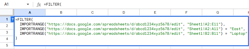
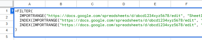
➤ To return only rows where Region is “East” and Product is “Laptop”, enter this formula in the target sheet (Filtered), cell A1:
=FILTER(IMPORTRANGE(“https://docs.google.com/spreadsheets/d/abcd1234xyz5678/edit”, “Sheet1!A2:E11”),IMPORTRANGE(“https://docs.google.com/spreadsheets/d/abcd1234xyz5678/edit”, “Sheet1!A2:A11”) = “East”,IMPORTRANGE(“https://docs.google.com/spreadsheets/d/abcd1234xyz5678/edit”, “Sheet1!B2:B11”) = “Laptop”)
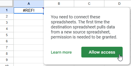
➤ Press Enter, and grant access when prompted.
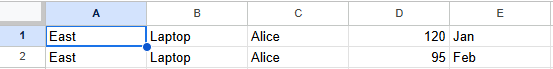
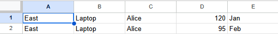
➤ The filtered rows will now appear based on the two criteria from the source sheet.

FILTER with Multiple IMPORTRANGE Calls
This method pulls in each column individually using separate IMPORTRANGE functions, allowing Google Sheets to filter values based on multiple criteria. It works well when you’re targeting specific columns and conditions, but it can become inefficient with large datasets.
These are the datasets we will be using to demonstrate the methods:
Source Sheet (Sales_Data):
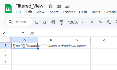
Target Sheet (Filtered):
Steps:
➤ Use the source dataset from the file Sales_Data, in cells A1:E11, with columns for Region, Product, Sales Rep, Units Sold, and Month.
➤ Copy the source file URL, for example:
https://docs.google.com/spreadsheets/d/abcd1234xyz5678/edit

➤ In the target sheet, enter the following formula in cell A1 to filter for rows where the Region is “East” and Product is “Laptop”:
=FILTER(IMPORTRANGE(“https://docs.google.com/spreadsheets/d/abcd1234xyz5678/edit”,”Sheet1!A2:E11″),IMPORTRANGE(“https://docs.google.com/spreadsheets/d/abcd1234xyz5678/edit”,”Sheet1!A2:A11″)=”East”,IMPORTRANGE(“https://docs.google.com/spreadsheets/d/abcd1234xyz5678/edit”, “Sheet1!B2:B11”) = “Laptop”)
➧ "Sheet1!A2:A11" brings in the Region column, while "Sheet1!B2:B11" brings in the Product column.
➧ FILTER returns only rows where Region = "East" and Product = "Laptop".
➤ Make sure to allow access the first time IMPORTRANGE is used.
➤ Once access has been provided, the IMPORTRANGE will display the filtered rows that meet both conditions.
Combine FILTER & INDEX Functions With Single IMPORTRANGE
This method uses a single IMPORTRANGE call to import the entire dataset and combines it with INDEX to apply filtering on specific columns. It’s more efficient than using multiple IMPORTRANGE calls, especially with larger datasets.
Steps:
➤ Use the source dataset from the file Sales_Data, in cells A1:E11, with columns for Region, Product, Sales Rep, Units Sold, and Month.
➤ Copy the source file URL, for example:
https://docs.google.com/spreadsheets/d/abcd1234xyz5678/edit

➤ In the destination file, enter the following formula in cell A1 to filter for rows where the Region is “East” and Product is “Laptop”:
=FILTER(IMPORTRANGE(“https://docs.google.com/spreadsheets/d/abcd1234xyz5678/edit”,”Sheet1!A2:E11″),INDEX(IMPORTRANGE(“https://docs.google.com/spreadsheets/d/abcd1234xyz5678/edit”,”Sheet1!A2:E11″),0,1)=”East”,INDEX(IMPORTRANGE(“https://docs.google.com/spreadsheets/d/abcd1234xyz5678/edit”, “Sheet1!A2:E11″), 0, 2) =”Laptop”)
➧ INDEX(..., 0, 1) targets the Region column (1st column), and INDEX(..., 0, 2) targets the Product column (2nd column).
➧ FILTER selects only rows where Region = "East" and Product = "Laptop".
➧ Only one IMPORTRANGE call makes this method more optimized than using separate ones.
➤ Press Enter to return all matching rows from the source sheet.

Use LET & FILTER Function with Single IMPORTRANGE
This method uses the LET function to store the imported data once and reuse it multiple times inside FILTER, improving formula clarity and performance. It’s ideal for advanced users working with multiple filter conditions on the same dataset.
Steps:
➤ Use the source dataset from the file Sales_Data, in cells A1:E11, with columns for Region, Product, Sales Rep, Units Sold, and Month.
➤ Copy the source file URL, for example:
https://docs.google.com/spreadsheets/d/abcd1234xyz5678/edit
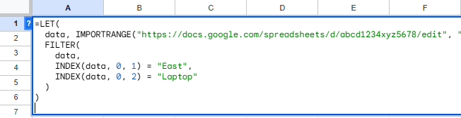
➤ In the destination file, enter the following formula in cell A1 to filter for rows where the Region is “East” and Product is “Laptop”:
=LET(data,IMPORTRANGE(“https://docs.google.com/spreadsheets/d/abcd1234xyz5678/edit”,”Sheet1!A2:E11″),FILTER(data,INDEX(data, 0, 1) = “East”,INDEX(data, 0, 2) = “Laptop”))
➧ INDEX(data, 0, 1) extracts the Region column, and INDEX(data, 0, 2) the Product column.
➧ FILTER uses these columns to apply both conditions efficiently.
➧ This method avoids repeating the IMPORTRANGE call, keeping your formula cleaner and faster.
➤ Press Enter to return the filtered results from the source file.
Utilize QUERY & IMPORTRANGE With Multiple WHERE Conditions
The QUERY function lets you apply multiple filter conditions in SQL-like syntax directly to data pulled using IMPORTRANGE. This is a powerful option when you want a more readable formula for multiple criteria.
Steps:
➤ Use the source dataset from the file Sales_Data, in cells A1:E11, with columns for Region, Product, Sales Rep, Units Sold, and Month.
➤ Copy the source file URL, for example:
https://docs.google.com/spreadsheets/d/abcd1234xyz5678/edit
➤ In the destination file, enter the following formula in cell A1 to filter for rows where the Region is “West” and Month is “Feb”:
=QUERY(IMPORTRANGE(“https://docs.google.com/spreadsheets/d/abcd1234xyz5678/edit”, “Sheet1!A1:E11”),“SELECT * WHERE Col1 = ‘West’ AND Col5 = ‘Feb'”,1)
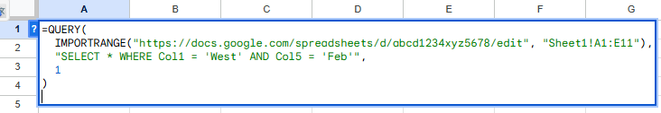
➧ QUERY uses Col1 for Region and Col5 for Month based on the column order.
➧ The SELECT * portion returns all columns where both conditions are met.
➧ 1 indicates that the first row of the range contains headers.
➤ Press Enter to retrieve all rows matching both conditions from the source sheet.

Frequently Asked Questions
Can I filter data from another Google Sheet without using IMPORTRANGE multiple times?
Yes, it’s best to avoid repeating IMPORTRANGE by assigning it once using the LET function. This improves performance and ensures consistent results across all conditions.
Why am I getting a “FILTER has mismatched range sizes” error?
This happens when the arrays used in the FILTER function don’t have the same number of rows. Often, it’s caused by inconsistent IMPORTRANGE calls or using an incomplete range reference in INDEX.
Do I need to click “Allow Access” every time I use IMPORTRANGE?
No. You only need to authorize access once per destination file and source file pair. After that, the connection is persistent unless the source file’s permissions change.
Can I use OR conditions in IMPORTRANGE filters?
Yes, but you’ll need to use a workaround like the plus sign (+) in the logical test inside FILTER, or switch to QUERY for more complex filtering with OR.
Wrapping Up
Filtering data from another Google Sheet using multiple criteria is fully possible with a smart combination of IMPORTRANGE, FILTER, INDEX, LET, and QUERY. While IMPORTRANGE alone brings data across files, combining it with filtering logic gives you precise control over what’s shown. Use LET for cleaner formulas, or QUERY when you prefer SQL-like conditions. Choose the method that fits your workflow best and keep your cross-file reporting dynamic, accurate, and automated.