Formatting cells in Google Sheets means modifying the visualization of the data in cells. You can make numbers look like money or dates look different. To do this, you have to select the cells you want to format, then click “Format” at the top. From there, you can choose options like “Number” to change how numbers appear, or “Date” to change how dates look. You can also change colors and styles to make the data easier to read. In this article, we’ll learn different aspects of formatting cells in Google Sheets.
What Is Formatting Cells in Google Sheets?
Formatting cells in Google Sheets refers to the process of customizing the appearance of data within those cells. This can include changing or modifying-
- Font style and size
- Text color
- Cell background color
- Number format
- Alignment (horizontal and vertical)
- Borders and gridlines
- Cell merging
- Text wrapping
- Conditional formatting
- Currency, date, and time formatting
Formatting Cells with Different Formatting Options
Now we’ll discuss different types of formatting options available in Google Sheets and see how they work with our particular dataset with no format initially.
Formatting Cells as Number in Google Sheets
When you enter numerical data in the cells of Google Sheets, this application automatically recognizes your data format and turns your entry into that format with conventional indentation and alignment. So, when you put a number in a cell, it’ll simply understand the number format and you don’t have to manually convert your data format to number again.
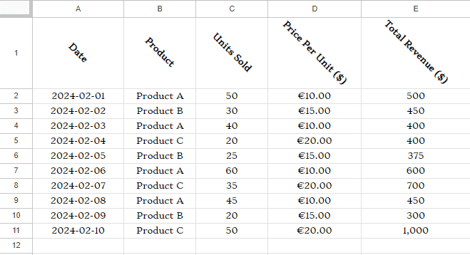
But you can again define the number format more specifically with decimals, scientific format, fractions, percentage or more other formats you want. Let’s consider the following dataset where all entries are in default format now.
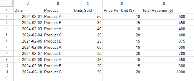
Here, if we want to change the format of the prices in Column D and add decimal points, what we have to do is:
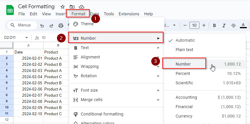
➤ Select the cells where you want to apply number format with decimal points.
➤ Go to the Menu bar and select Format > Number > Number.
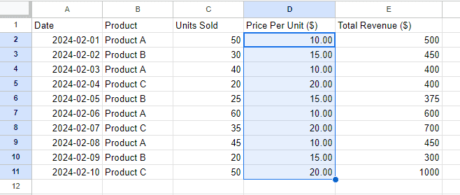
And in the following image, we see now the prices in Column D are with decimal points.
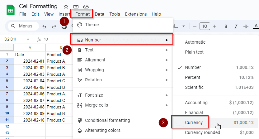
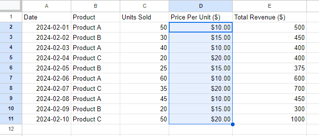
You can also apply more other number formats from the options. Let’s format these prices now by adding currency symbols before the digits. To format cells or numbers with currency symbols, do the following steps:
➤ Select the cells that you want to convert into currency format.
➤ From the Menu bar, select Format > Number > Currency.
And all the numbers in Column D have a dollar sign before each of them.
You can also customize the currency symbol and choose different currency. To do this:
➤ Select the cells from your dataset.
➤ From the Menu bar, go to Format > Number > Custom Currency.
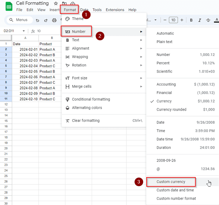
➤ From the Custom currencies tab, select the currency option you want.
➤ Press Apply and you’re done.
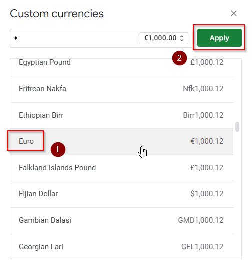
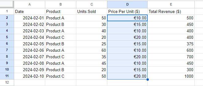
This is how you can easily change the default currency format and choose your desired one from the list.
Custom Number Format
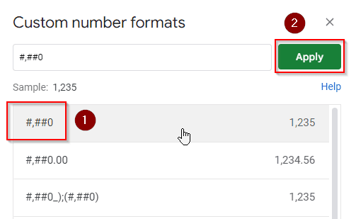
By using the Format menu, you can also change the date and time formats with more customizations. There is a Custom Number Format option too where you can create a custom format for zip codes, telephone numbers, and more. Let’s say, we want to add a comma for a thousand separator in a number. What you have to do is:
➤ Select the cells to apply custom number format.
➤ From the menu bar, go to Format > Number > Custom Number Format.
➤ From the list of number format, choose #,##0 and press Apply.
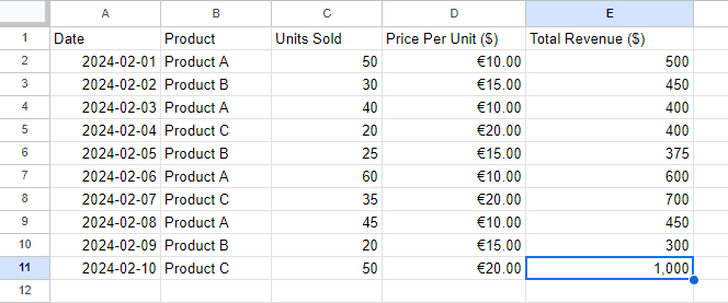
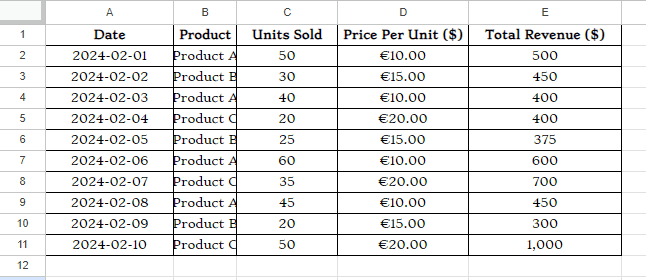
Look at the following image, in Cell E11, the value 1000 has a comma for thousand separator.
Formatting Cells as Text in Google Sheets
When you format a cell as text in Google Sheets, it’ll be in plain text format. That means you can type anything in the cell and it will be treated as text only. The alignment will be fixed for text format, and if you put numbers or dates in those cells you cannot make any calculations with those cells either. Formatting cells as text is needed when you want to type anything and keep exactly in the format you typed.
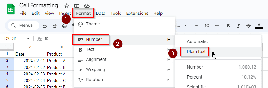
To convert a range of cells of numbers into text format, do the following steps:
➤ Select the cells that you want to turn into text format.
➤ From the menu bar, go to Format > Number > Plain Text.
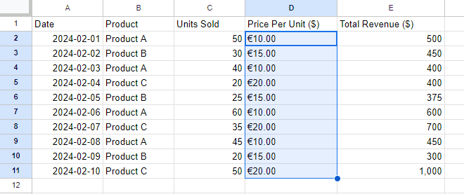
Here, we’ve converted the prices into text format. And the alignment of the cells have changed to the left because the text format keeps the data with left alignment only.
Changing Font in Google Sheets
We can change both the font type and font size in Google Sheets. If you want to choose a different font type, follow the steps below:
➤ Select the data where you want to apply different font type.
➤ From the toolbar, choose the Font options and select any font you want.
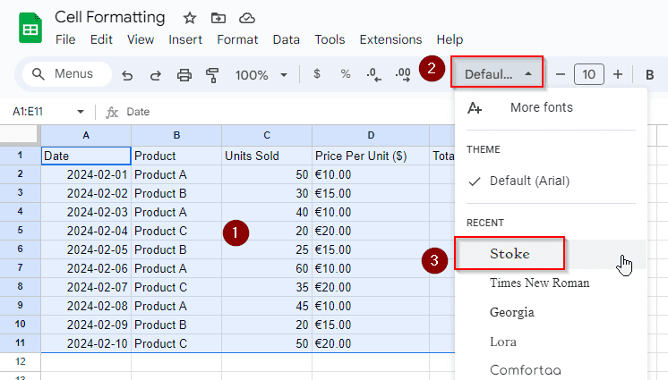
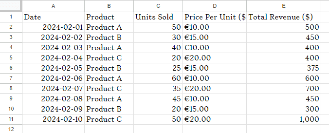
The data in new font will look like the following as I chose Stoke:
If you want to increase or decrease the font size, you have to do the following:
➤ Select the cells where you want to change the font size of the data.
➤ From the menu bar, select Format > Font Size > (choose any size you want)
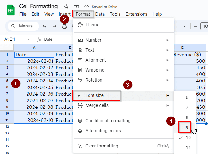
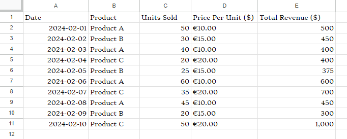
Here, we’ve reduced the font size to 9 which was 10 before, so our data with new look will be the following with the decreased font size.
How to Change Text Alignment in Google Sheets
Alignment in Google Sheets refers to the positioning of text or numbers within a cell. It determines whether the content is aligned to the left, right, or center of the cell horizontally, and whether it’s aligned to the top, bottom, or middle of the cell vertically.
Horizontal Alignment
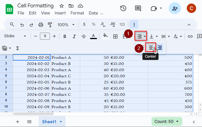
Let’s say we want to center the text by changing its alignment. What we have to do is:
➤ Select the data.
➤ From the toolbar, select Horizontal Alignment > Center.
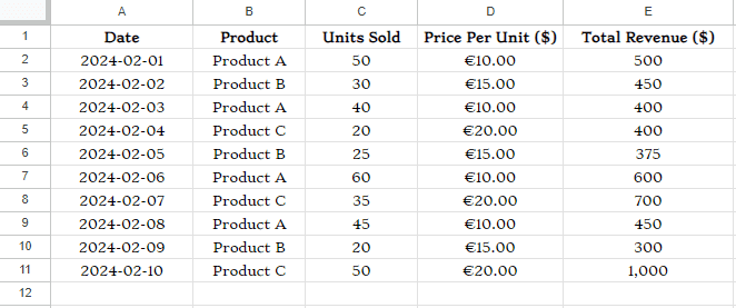
And all the selected data are now center aligned as shown below.
Vertical Alignment
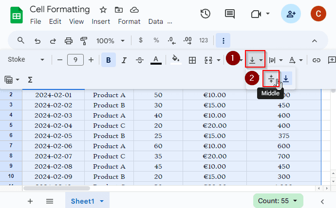
Vertical alignment has also 3 options- top, middle and bottom. By default, in Google Sheets, all data are bottom aligned. If we want to change it to middle align, we have to follow the steps below:
➤ Select the data first.
➤ From the toolbar, select Vertical Alignment > Middle.
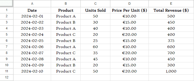
And all the data are now middle aligned which seems not making much difference with the previous format. For larger row heights, the difference between the vertical alignments will be more understandable.
Changing Indent in Google Sheets
Indentation of text in Google Sheets refers to adjusting the space between the cell border and the text within the cell. There is no built-in option in Google Sheets to change the indent of a text in a cell. But we can do this by applying a custom number format. Let’s consider another dataset here:
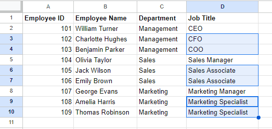
Suppose, we want to increase the indent of the selected job titles so we can easily understand these roles are the subordinates of the CEO, Sales Manager and Marketing Manager. To change the indent of the text, we have to follow the instructions below:
➤ Select the cells with data for applying indentation.
➤ From the menu bar, select Format > Number > Custom Number Format.
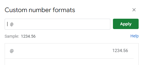
➤ In the Custom Number Format, put spaces in the editor before typing ‘@’. The number of spaces will define the indent size.
➤ Press Apply and you’re done.
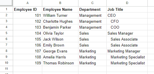
And the selected texts in Column D have indents in front of them now.
Rotating Text in Google Sheets
Rotating text in Google Sheets means changing the orientation of text within a cell. This allows you to display the text vertically or at an angle, rather than horizontally. Rotating text can be useful for fitting long labels into narrow columns or creating headers that span multiple lines. To rotate the text in Google Sheets, let’s follow the steps below:
➤ Select the texts or data in the cells.
➤ From the menu bar, go to Format > Rotation > (Choose any rotation option you want)
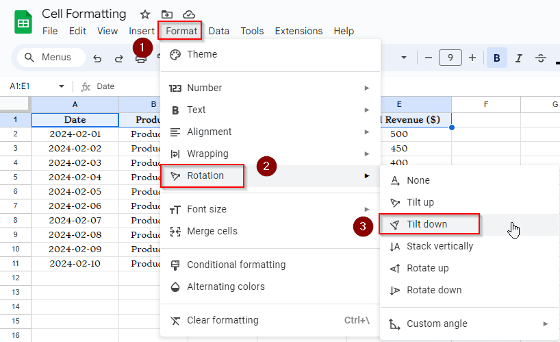
And the selected data will look like the following as we’ve chosen the option Tilt down here.
You can also specify the rotation angle from Custom Angle options. To do this, you have to select the data first and then go to Menu bar > Format > Rotation > Custom Angle > (choose the angle you want).
Adding Borders in Google Sheets
In Google Sheets, a cell border is like a line that goes around the edges of a cell. It helps to separate one cell from another. You can add borders to cells to make your data look more organized and easier to read. It’s like drawing lines around the edges of each cell to create a grid. To add border around the cells, do the following:
➤ Select the cells you want to add borders around.
➤ From the toolbar, go to the Borders option > All Borders.
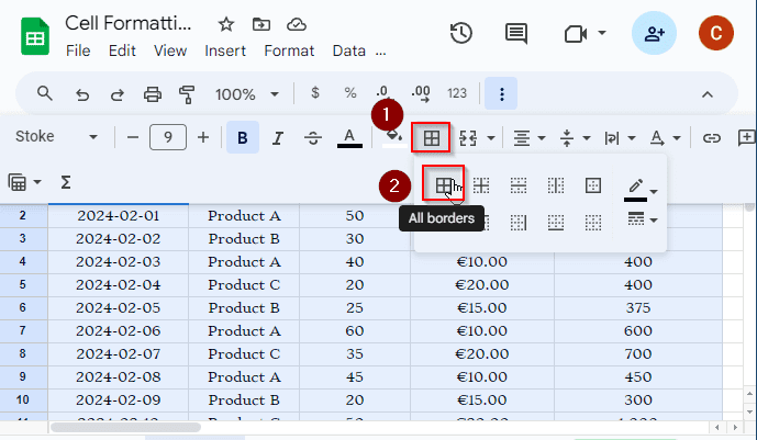
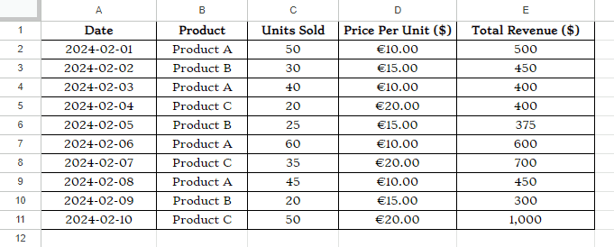
And the cells you selected have all borders around them.
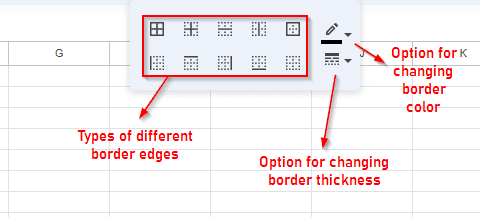
You can also add more other types of borders like- inner, outer, horizontal, vertical, top, bottom, left and right borders according to your requirements. Not only that, you can again increase the thickness of your borders or change the default border color from the Border options. But if you see green-colored borders around cells or a column, then there might need some fixes since they are not part of built-in border formats.
How to Fit Text to a Cell in Google Sheets
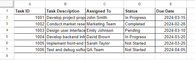
Fitting text to cells in Google Sheets means adjusting the size of the text so that it fits entirely within the width and height of the cell. This ensures that the entire text is visible without spilling over into adjacent cells. It’s useful for making sure your data looks neat and is easy to read, especially when dealing with cells of different sizes or limited space. Look at Column B in the following image. The texts are not fitted properly. You can make all cells the same sizes or there are some other ways around too.
To fit the text to cells properly in Google Sheets, we have follow the steps below:
➤ Select the cells first that you want to adjust for fitting the text inside.
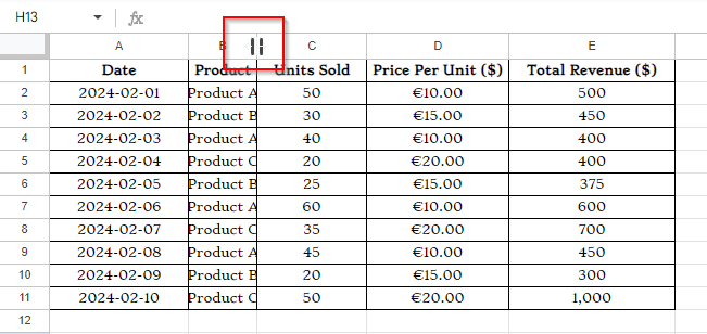
➤ Move your mouse cursor to the column headers under which your text data needs to be fitted to the cells.
➤ Double-click on the vertical expansion bar in the left or right as shown in the image below.
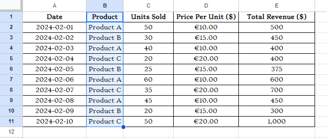
And the texts in the selected column are now fitted properly to the cells.
You can also specify the width of the columns by choosing Resize Column options. To do this:
➤ Select the entire column by clicking on the header of that column.
➤ Right click on the mouse and open the Context Menu.
➤ From the options, select Resize Column.
➤ Enter the width in pixels and click OK.
Again, you can select all the columns together that contain text and resize them by following the similar procedures. Or if you don’t want to resize manually, you can simply select the column headers of all the columns and autofit the text to the cells by double-clicking on the expansion bar in the column headers.
Wrapping Texts in Cells to Make Multiple Lines
Wrapping text in Google Sheets means allowing text to automatically move to the next line within a cell if it exceeds the cell’s width. This feature ensures that all the text remains visible within the cell without being cut off. It’s helpful for displaying lengthy text entries or long sentences without enlarging the cell width, making your data more readable and organized.
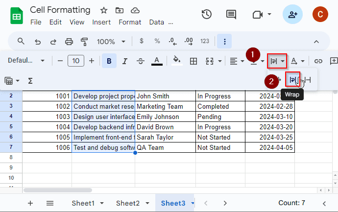
Let’s consider the following dataset where in Column B, the texts need to be wrapped within the cells.
To wrap text in cell, what we have to do is:
➤ Select the cells for wrapping text inside.
➤ From the toolbar, go to Text Wrapping option > Wrap.
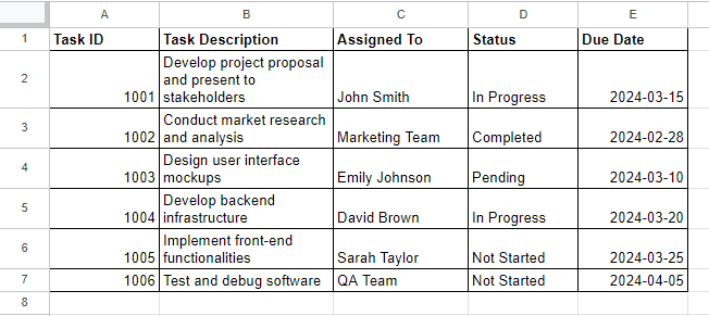
Now the cells you selected are formatted for wrapping texts as shown below.
Adding Cell Background Color in Google Sheets
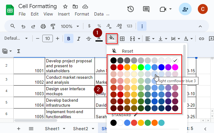
You can also add the background color in the cells to make them visually better. This feature allows you to highlight important data, categorize information, or simply improve the aesthetics of your Excel worksheet. To add the background color of cells in Google Sheets, let’s follow the steps below:
➤ First select the cells where you want to add or fill color.
➤ From the toolbar options, go to Fill Color > (Choose the color you want)
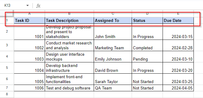
The selected cells are now filled with the color you chose.
Frequently Asked Questions
How do I Autosize cells in Google Sheets?
To autosize all cells in Google Sheets, select all the cells and then drag your mouse cursor between any two column letters, double click on the vertical line with horizontal arrows and all of your cells will be autosized.
Can you copy cell formatting in Google Sheets?
Yes, you can copy only the cell formatting in Google Sheets. To do that, copy a cell first, select another cell where to paste, open the context menu and choose Paste special > Format only. Or you can also use the keyboard shortcuts Ctrl + Alt + V to paste as format only in the destination cell.
What is paint format?
Format painter is a tool in Google Sheets to copy and paste the format of a cell in another location. Suppose, you want to copy the format of cell A1 to B1. Now select the cell A1, click on the Format painter option from the toolbar and then click on cell B1. The format of cell A1 will be copied to cell B1.
What is clear formatting in Google Sheets?
The Clear formatting option in Google Sheets enables us to clear all types of format from a cell. You can use this option by selecting a cell first where you want to clear all types of format and from the menu bar then choose Format > Clear formatting. Your selected cell will contain no formats anymore.
Concluding Words
In conclusion, formatting cells in Google Sheets is essential for organizing and presenting data effectively. By changing text alignment, fonts, and adding borders, you can enhance readability. Adjusting cell indentation and rotating text offer additional customization options. Fitting text to cells and wrapping text ensure all content remains visible. Moreover, adding background color can help emphasize important information or categorize data. Overall, mastering these formatting features empowers users to create visually appealing and well-organized spreadsheets in Google Sheets.