The number format in Google Sheets is used to control the appearance of the numerical values in cells. It lets us customize the number format with decimal, percentage, fraction, currency and more. There are several types of default formatting options associated with the number format in Google Sheets. We can also create a unique number format according to our requirements. In this article, we’re going to learn about the functions of this number format as well as how we can use and customize them for our various needs.
What Is Number Format in Google Sheets?
Number format in Google Sheets is how numbers look in cells. It helps to show numbers in different ways, like with decimals, as currency, or as percentages. It’s like defining how numbers appear so they’re easier to read and understand.
Different Types of Number Format in Google Sheets
In Google Sheets, there are several types of number formats available:
- Number: This format displays numbers as they are, without any special formatting. It includes integers and decimals with default format.
- Currency: The currency format will let you add a currency symbol before the number. By default, it adds a dollar ($) sign only, but you can also customize the currency format and choose the currency symbol of any country you need.
- Accounting: Almost similar to the currency number format but here the negative values are enclosed within parentheses to show differences with the positive values.
- Percentage: Displays numbers as percentages automatically by multiplying them with 100 and adding a percentage symbol (%).
- Date: Formats numbers as dates, showing them in various date formats like MM/DD/YYYY or DD/MM/YYYY.
- Time: Formats numbers as time, displaying them in hours, minutes, and seconds.
- Scientific notation: Represents numbers in scientific notation and shows them as a coefficient multiplied by 10 raised to a power.
- Duration: Formats numbers as durations of time, displaying them in hours, minutes, and seconds or as days.
- Custom: Allows users to create their own custom number formats based on specific preferences or requirements.
Examples of All Number Formats in Google Sheets
Now we’ll explore one by one with examples of all types of number format in Google Sheets.
Basic Number Format
The basic number format in Google Sheets is the default way the numbers are displayed in cells without any additional formatting. It simply shows the numbers as they are, without adding any currency symbols, percentages, or decimal places. When you put an integer or a decimal value in a cell in Google Sheets, it will by default format it as a number and align the value to the right since right alignment is used for default number format in a cell here.
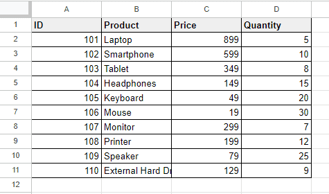
Let’s consider Columns C and D in the following dataset. Here only simple number format has been used by Google Sheets.
Currency Number Format
In Google Sheets, the currency number format is a way to display numbers like money. It adds the currency symbol, such as $, €, or £, before the number. You can also choose how many decimal places to show. It’s helpful for showing financial data or prices in a clear and recognizable way.
To format numbers with currency symbols, what you have to do is:
➤ Select the cells where you want to apply currency format.
➤ From the menu bar, go to Format > Number > Currency.
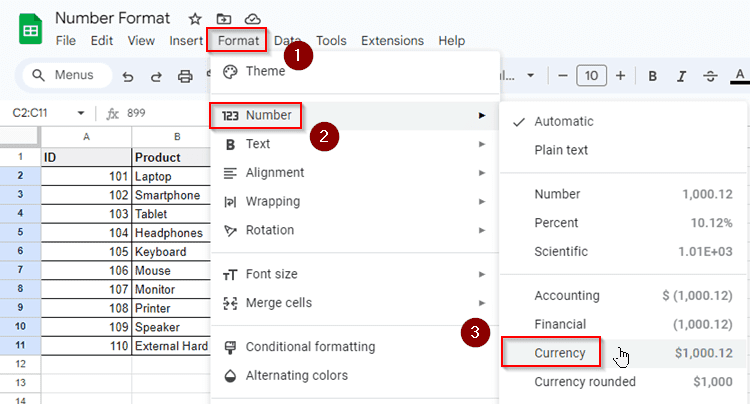
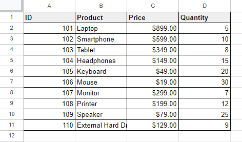
And the selected cells will be formatted with the dollar symbol ($).
If you need to add other currency symbols like euro or pound, you have to switch to custom currency formatting which will be explained in the Custom Number Formatting section in this article.
Accounting Number Format
The accounting number format in Google Sheets is used to make financial data easier to read and understand. It aligns the currency symbols and decimal points in a column, which makes it simpler to compare numbers and follow them across the spreadsheet. This format is commonly used in financial statements, budget sheets, and any other documents where accurate representation of monetary values is important.
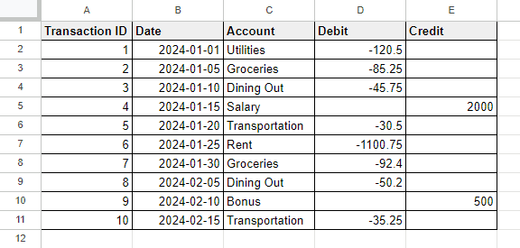
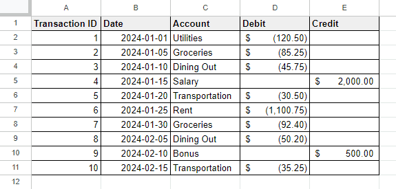
Let’s have a look at another dataset here with debit credit columns. When we apply accounting number format in these two columns the dollar symbol will be added to the numbers automatically and the negative numbers will be shown in parentheses.
To apply accounting number format in Google Sheets:
➤ Select the cells where you need to apply an accounting format.
➤ From the menu bar, select Format > Number > Accounting.
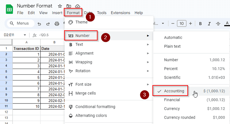
Here we’ve applied the accounting format in the Debit and Credit columns. And the output is shown in the picture below:
Percentage Format
In Google Sheets, the percentage format is used to show numbers as percentages. It converts the numbers into a percentage by multiplying them by 100 and adding a percentage sign (%). This format is helpful when you want to display values as percentages, such as when working with percentages of scores, discounts, or growth rates.
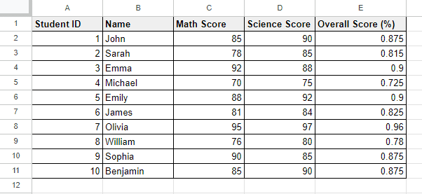
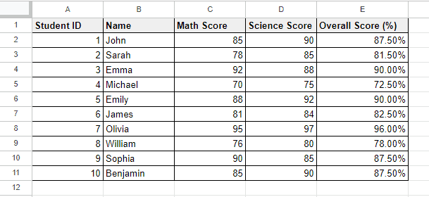
Suppose we have a dataset like below where we want to know the marks percentage for all subjects.
To convert the decimals or numeric values to percentage, let’s do the following:
➤ Select the cells where you have to apply a percentage symbol.
➤ From the toolbar, select the Format as Percentage option.
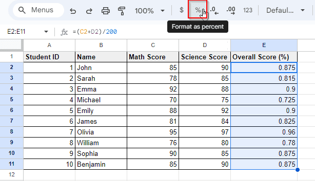
Now our selected numerical data will be converted into percentage format with the percentage symbols.
Scientific Notation Format
Scientific notation is a way of writing numbers that are very large or very small using powers of 10. It’s a shorthand method where a number is expressed as a coefficient multiplied by 10 raised to a power. This notation helps to represent numbers more concisely and makes it easier to work with extremely large or tiny values in mathematics, science, and engineering.
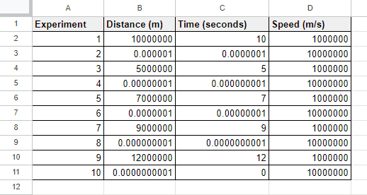
In the following dataset, the numbers are very long and we can’t easily read them or understand the tenths of the digits. But if we convert these numbers into scientific format, it’ll be much easier to read as well as know the differences among the numbers.
To convert numbers into scientific form or notation, follow the steps below:
➤ Select the cells where you need to convert the numbers into scientific notations.
➤ From the menu bar, go to Format > Number > Scientific.
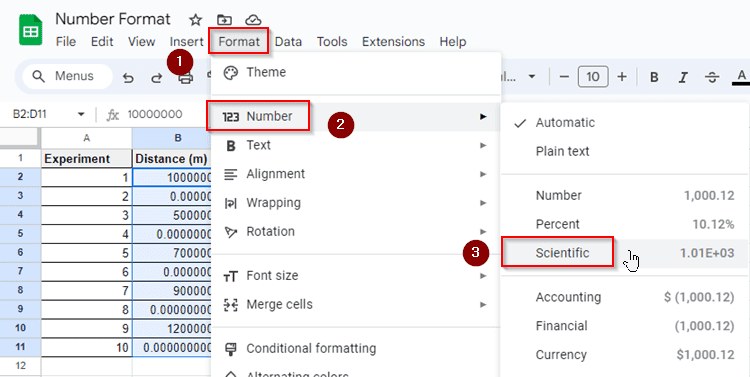
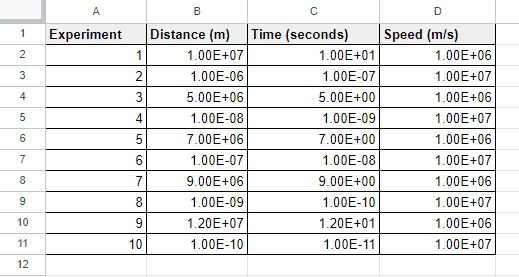
And the selected numbers will be now shown in scientific format or notations.
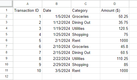
Date Format
In Google Sheets, there are various types of date formats available to display dates in different ways. These formats include options like “Month/Day/Year” (e.g., 02/19/2024), “Day/Month/Year” (e.g., 19/02/2024), “Day, Month Year” (e.g., February 19, 2024), and “Year-Month-Day” (e.g., 2024-02-19).
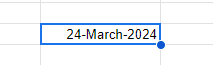
You can manually type a date in lots of different formats and in most cases, Google Sheets will automatically identify your chosen date format. This is a big advantage here! For example, we can type “24-March-2024” in a cell. And Google Sheets will recognize it as the date format automatically.
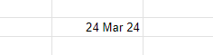
The value with text and numbers we have typed in the cell is automatically right aligned and Google Sheets shows dates with right alignment. You can also try with other date formats like- “24 Mar 24”, Google Sheets will recognize this date format too.
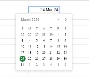
You can also change dates from here by double clicking on the date and choose another date from the date picker.
Now sometimes the dates can be in normal number format which means the date can be present as its datevalue or serial number. Each date has its own serial number in Google Sheets, like- 24 March 2024 has its date serial number 45375. To convert this serial number to a proper date format what you have to do is:
➤ Select the cell with the date serial number or the datevalue.
➤ From the menu bar, go to Format > Number > Date.
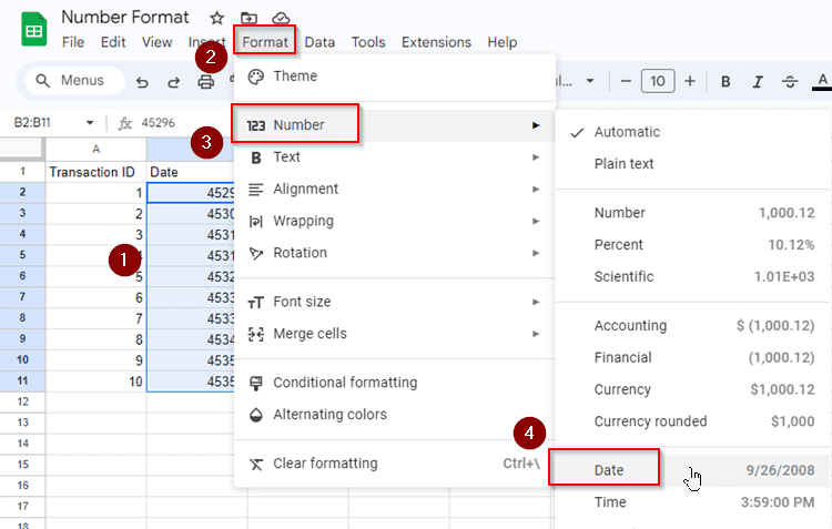
And the date serial numbers will be formatted as real dates.
Time Format
In Google Sheets, there are several types of time formats available to display time in different ways. These formats include options like “Hour:Minute AM/PM” (e.g., 9:30 AM), “Hour:Minute:Second AM/PM” (e.g., 9:30:15 AM), and “Hour:Minute:Second” in 24-hour format (e.g., 09:30:15). Users can also customize time formats further by selecting options like displaying milliseconds or adding leading zeros for single-digit hours, minutes, or seconds.
Like date format, here you can too manually type a time and Google Sheets will recognize your time format. And again here all time value has its own serial number with decimals. For example, the time “6:45:52 P.M.” has its own time serial number 0.7818518519. And to convert this value to actual time format, what you have to do is:
➤ Select the cell with the time value.
➤ From the menu bar, go to Format > Number > Time and you’re done!
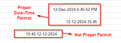
Google Sheets also allows you to input both date and time in a single cell with a proper format. To do this you have to type the date first in any format and then you can type the time with its format. But if you type time before the date, Google Sheets will not recognize it as date-time format and consider it as plain text value.
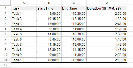
Duration Format
In Google Sheets, the duration format is used to represent the length of time in a particular format. It allows users to display time durations, such as hours, minutes, and seconds, in a consistent format. This format is helpful for tracking time intervals, durations of events, or elapsed time between two points.
Let’s have a look at the following example. In Column D, we’ve subtracted the Start Time from the End Time. Since the Start Time and the End Time both are in proper time format, after subtraction between them, the time duration has been formatted automatically by Google Sheets.
Duration time has also similar serial numbers like time values and date values. To convert this serial number to duration, we have to do the following:
➤ Select the cells where you have to apply duration format.
➤ From the menu bar, go to Format > Number > Duration.
Custom Format
There are three criteria of custom format in Google Sheets and they are:
➤ Custom Currency
➤ Custom Date and Time
➤ Custom Number Format
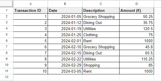
Custom Currency Format
In Google Sheets, the custom currency format allows users to customize how currency values are displayed in the spreadsheets. It enables users to specify the currency symbol, choose the number of decimal places, and format negative numbers, among other options.
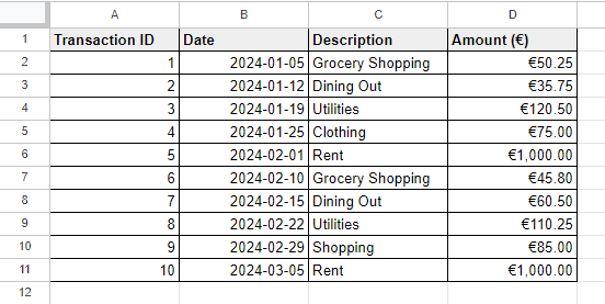
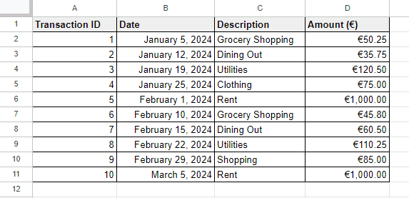
In the following dataset, we’ll add the currency symbol Euro (€) before the amounts in Column D.
To add Euro (€) or any other currency sign by using Custom currency, we have to follow the steps below:
➤ Select the cells first where you have to add Euro (€) or any other currency sign.
➤ From the menu bar, go to Format > Number > Custom Currency.
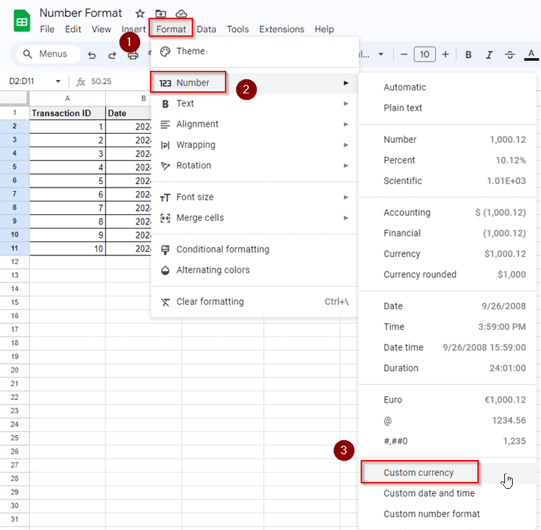
➤ In the text editor of the Custom Currencies tab, type the name of the currency and you’ll find the currency options with its symbol.
➤ Select the currency option from the list and click Apply.
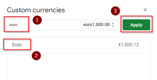
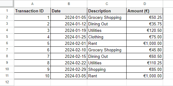
Now your selected cells are formatted with custom currency symbols.
Custom Date and Time Format
By using the Custom Date and Time Format option, you can select a particular format from a list of various date and time formats. For example, we have a dataset like the following where we want to change the date format.
To customize the date or time format, what we have to do is:
➤ Select the cells that contain dates or times or both.
➤ From the menu bar, go to Format > Number > Custom date and time.
➤ From the ‘Custom date and time formats’ tab, select a particular date time format you prefer.
➤ Click Apply and you’re all done.
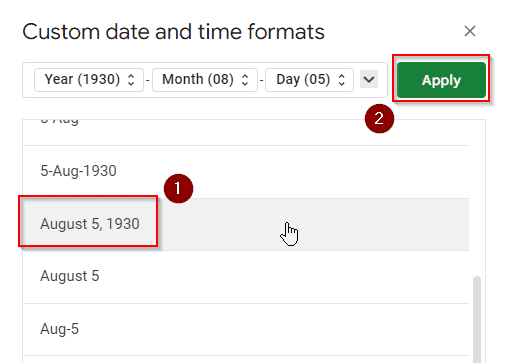
This is how we can easily change a date or time or date-time format according to our requirements.
Custom Number Format
In Google Sheets, custom number format is used to format numbers in a customized way according to the specific requirements. It enables users to control how numbers are displayed by specifying various elements such as formatting millions or thousands with abbreviations, adding commas between numbers, customizing decimal separators, converting all negative numbers to positive, adding phone number format, writing mixed fractions etc. Here, we’ll show you two examples of Custom Number Format in Google Sheets.
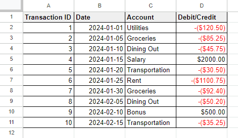
Example 1: Making Negative Numbers Red
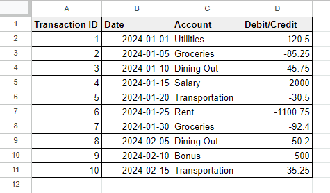
Let’s consider a dataset here. In the Debit/Credit column, we’ll turn all the negative numbers red.
To make all negative numbers red in Google Sheets, we have to do the following:
➤ Select the cells first.
➤ From the menu bar, go to Format > Number > Custom number format.
➤ In the new tab of the Custom number formats, type- $0.00;[Red]-($0.00).
➤ Click Apply.
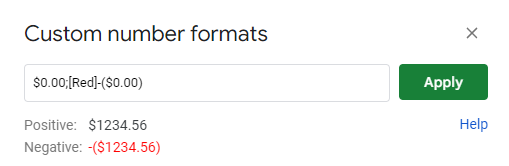
And now all negative numbers in the selected cells have turned into red as shown below:
Example 2: Adding Leading Zeros in a Number Format
Now we’ll deal with another example where we have to add leading zeros keeping the number format. In the following dataset, we want to add employee IDs as 001, 002, etc. But with the default number format, we are unable to do this. So we have to use the custom number format here.
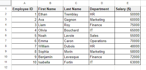
To add leading zeros keeping the number format properly, let’s follow the steps below:
➤ Select the cells where you have to add leading zeros in the numerical values.
➤ From the menu bar, choose Format > Number > Custom number format.
➤ In the input box of the Custom number format tab, type a certain number of zeros so that the numbers you have to format will contain the same number of digits. For example, if you want to add only one 0 before 12 (012), then type 000, or if you want to add two 0’s before 12 (0012) then type 0000.
➤ Click Apply and you’re all done.

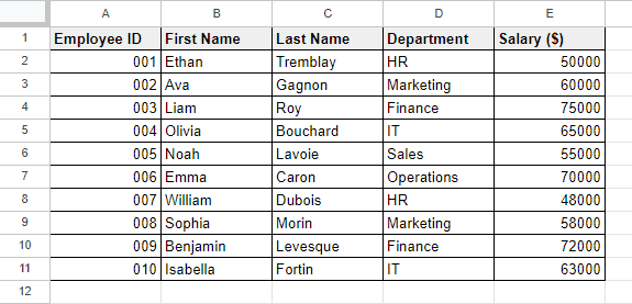
Now all the employee IDs have the leading zeros as well as the same number of digits.
How to Change or Convert Number Format in Google Sheets
Changing or converting a number format in Google Sheets to another particular number format is very simple. For example, if you need to convert the number format into text format, you have to do the following:
➤ First select the cells that you want to format as text.
➤ From the menu bar, choose Format > Number > Plain Text.
Similarly, you can also convert numbers to text, dates, decimals, percentages, scientific notations and more. Again you can convert a number stored as text to the proper number format from the Format options with few simple steps.
Frequently Asked Questions
How do I automatically format numbers in Google Sheets?
When you input a numeric value in Google Sheets, it’ll automatically recognize your input as a number format. If your cell is not in number format but contains a numeric value, you can select the cell and from the menu bar, choose Format > Number > Automatic. Google Sheets will now recognize the cell as a number format automatically.
How do I show 1000 as 1k in Google Sheets?
To show 1000 as 1k in Google Sheets, you have to use the custom number format. To do that:
➤ Select the cell first.
➤ Go to the menu bar and select Format > Number > Custom number format.
➤ In the editing field, type “0,\k” and then press Apply.
➤ Now the number 1000 will show as 1k in the cell.
What is the default Number format in Google Sheets?
The default number format in Google Sheets is Automatic.
How do I type 0000 in Google Sheets?
To type 0000 in Google Sheets, you have to use the custom number format. Select the cell first and then from the menu bar, select Format > Number > Custom number format. Now type “0000” (without quotes) in the editing field and press Apply. Now you can type 0000 in that cell in Google Sheets. 123 will become 0123, 12 will become 0012 and 1 will appear as 0001 there.
How do I add 0 to a zip code in Google Sheets?
To add 0 to a zip code in Google Sheets, you have to use the custom number format. Select the cell with a zip code first and then from the menu bar, select Format > Number > Custom number format. Now type “00000” (without quotes) in the editing field and press Apply. It’s applicable for e 5 digit zip/postal code with 00567, 05678 or 56789 format having leading zeros.
Concluding Words
In conclusion, Google Sheets offers a variety of number formats to suit different needs when working with data. These formats include basic numbers, currency, accounting, percentages, scientific notation, dates, times, durations, and custom formats. Each format serves a specific purpose, from representing financial data accurately to displaying time intervals or customizing how numbers are shown. By understanding and utilizing these formats effectively, we can enhance the readability and clarity of the spreadsheets.