When we work with large or changing datasets, using a regular VLOOKUP can become inefficient because cell ranges must be updated manually. A dynamic VLOOKUP solves this problem by automatically adjusting the lookup range when new data is added. This technique is commonly used in financial reports, sales trackers, and dashboards that are frequently updated.
To use a dynamic VLOOKUP in Excel, follow these steps:
➤ Create a named range or use a dynamic table to store your data.
➤ Apply the VLOOKUP formula using a dynamic range name.
➤ Test your formula by adding new rows or columns. The VLOOKUP will automatically adjust.

In this article, we will describe how to use a dynamic VLOOKUP in Excel using Dynamic VLOOKUP with Match, Column Reference, and Columns functions.
What Is a Dynamic VLOOKUP in Excel?
A dynamic VLOOKUP is an advanced version of the standard VLOOKUP formula that updates automatically when new data is added or removed. Instead of defining a fixed lookup range, you can create a dynamic named range using functions such as OFFSET or INDEX, which adjust based on the number of entries.
Using a Dynamic VLOOKUP with the MATCH Function
The Dynamic VLOOKUP with MATCH method enables us to look up data from multiple columns dynamically, eliminating the need to adjust the column index in our VLOOKUP formula manually. Instead of fixing the column number, the MATCH function determines the column index automatically based on our input. We use this method for datasets with expanding or changing columns, usually useful in monthly sales or performance reports.
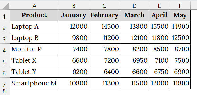
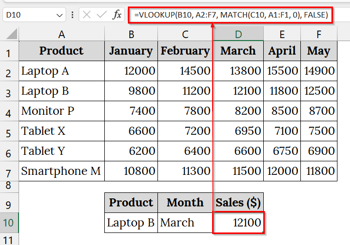
We have a dataset that contains product sales of BrightVision Electronics over five months. We will use a dynamic VLOOKUP with the MATCH function to dynamically retrieve sales data for any product and month without rewriting the formula each time.
Steps:
➤ Open your worksheet that contains your data. For example, we have taken a dataset that contains Product in Column A, monthly sales of January in Column B, February in Column C, March in Column D, April in Column E, and May in Column F.
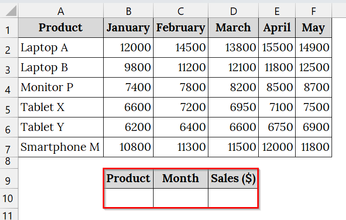
➤ In another section of your worksheet, use three cells:
- B10 for the selected product (e.g., “Laptop B”)
- C10 for the selected month (e.g., “March”)
- D10 to see the sales for the selected product and month.
➤ In cell B10 and C10, type the selected product and month name. For example, type Laptop B in cell B10 and March in C10.
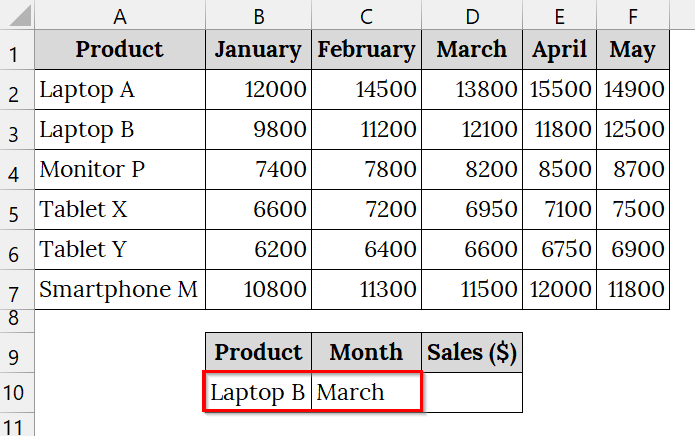
➤ Click on cell D10 to display the result for the selected product and month.
➤ Type the following formula:
=VLOOKUP(B10, A2:F7, MATCH(C10, A1:F1, 0), FALSE)
➤ Press Enter. The result will appear as 12100 in cell D10.
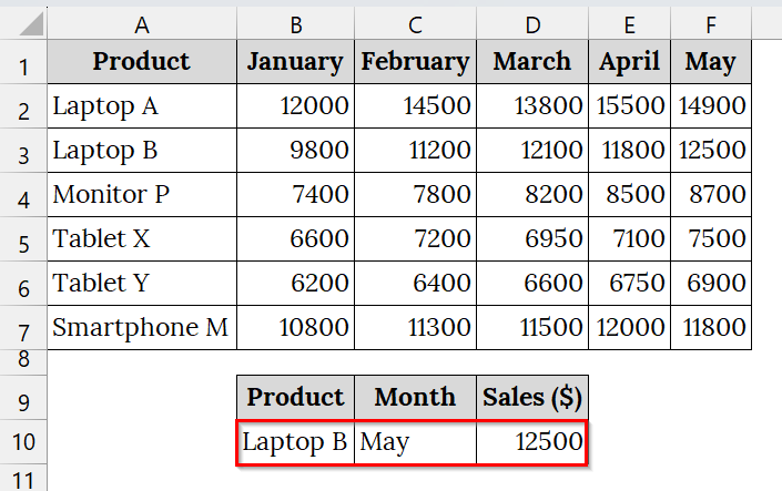
➤ Change the value in C10. For example, switch from “March” to “May” and watch the result automatically update. This demonstrates the formula’s dynamic flexibility.
Note:
➥ Ensure your month names in the top row (A1:F1) exactly match the input values; otherwise, the MATCH function may return an error.
➥ The MATCH function helps you avoid hardcoding column numbers, making your VLOOKUP formula easier to maintain.
➥ You can expand this approach to yearly or regional data simply by adjusting the lookup range and header references.
Applying the VLOOKUP with a Dynamic Column Reference
The VLOOKUP with a dynamic column reference method helps in dynamic lookups across multiple columns by using the COLUMN function to automatically adjust the column index in a VLOOKUP formula. Compared to the MATCH-based method, this method is easier when copying across columns but less flexible if column headers change.
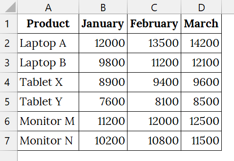
We have a dataset that contains monthly sales data for a specific product. Instead of writing multiple VLOOKUP formulas with different column indexes, we will use a dynamic column reference approach to fetch January, February, and March sales with one easily extendable formula.
Steps:
➤ Open your Excel sheet that contains your data. For example, we have taken a dataset that contains Product in Column A, the monthly sales of January in Column B, February in Column C, and March in Column D.
➤ In the section below of your worksheet, reserve four cells according to your header:
- A10 for the selected product.
- B10 for the sales of January.
- C10 for the sales of February.
- D10 for the sales of March.
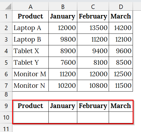
➤ In cell A10, type the selected product. For example, type Tablet X in cell A10.
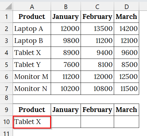
➤ Click on cell B10 to display the result for the selected product.
➤ Type the following formula:
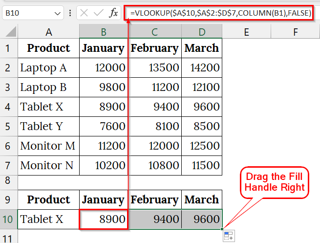
=VLOOKUP($A$10,$A$2:$D$7,COLUMN(B1),FALSE)
➤ Press Enter. The result will appear as 8900 in cell B10.
➤ Drag the Fill Handle rightwards to fill across the months. You will notice the formula automatically adjusts the column reference because of the COLUMN function.
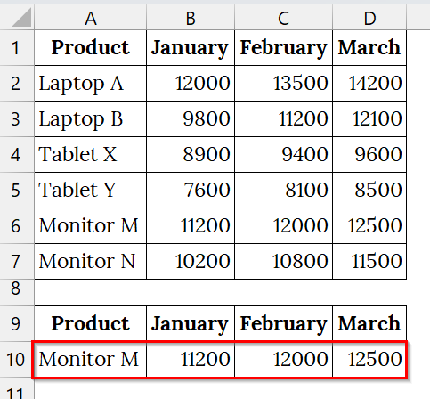
➤ Change the value in A10. For example, type Monitor M and watch the result automatically update. This demonstrates the formula’s dynamic flexibility.
Note:
The COLUMN function dynamically returns the column index, avoiding manual index adjustments.
Using the VLOOKUP with the Excel COLUMNS Function
The combination of the VLOOKUP and COLUMNS functions makes our lookup formula dynamic. Instead of manually changing the column index each time, the COLUMNS function automatically counts how many columns are in our range and updates the VLOOKUP output as we drag the formula horizontally.
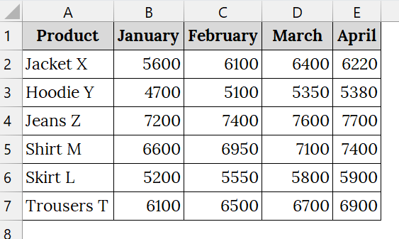
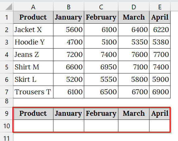
We have a dataset that contains monthly sales of various clothing products for the first quarter of the year. We will use VLOOKUP with the COLUMNS function to dynamically retrieve the sales data for any selected product for all months.
Steps:
➤ Open your worksheet that contains your data. For example, we have taken a dataset that contains Product in Column A, the monthly sales of January in Column B, February in Column C, March in Column D, and April in Column E.
➤ In the section below of your worksheet, reserve five cells according to your header:
- A10 for the selected product.
- B10 for the sales of January.
- C10 for the sales of February.
- D10 for the sales of March.
- E10 for the sales of March.
➤ In cell A10, type the selected product name. For example, type Skirt L.
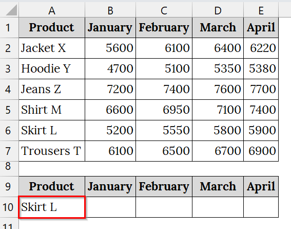
➤ Click on cell C10 to display the result for the selected product.
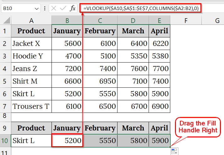
➤ Type the following formula:
=VLOOKUP($A10,$A$1:$E$7,COLUMNS($A1:B2),0)
➤ Press Enter. The result will appear as 8900 in cell B10.
➤ Drag the Fill Handle right side to fill across the months. You will notice the formula automatically adjusts the column reference because of the COLUMN function.
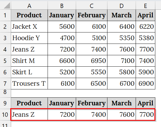
➤ Change the value in A10. For example, type Jeans Z and watch the result automatically update. This demonstrates the formula’s dynamic flexibility.
Frequently Asked Questions
Why should I use a dynamic VLOOKUP instead of a normal VLOOKUP?
Because it saves time and prevents errors when your data expands frequently.
Can I use dynamic VLOOKUP with tables?
Yes! Converting your range into an Excel Table automatically makes it dynamic.
Which is better: dynamic VLOOKUP or INDEX-MATCH?
INDEX-MATCH is often more flexible, but a dynamic VLOOKUP is simpler for most users.
Do dynamic ranges slow down Excel?
Not significantly, but for very large datasets, using Excel Tables is more efficient.
Concluding Words
Dynamic VLOOKUP helps you create flexible, error-free Excel formulas that grow with your data. Through dynamic VLOOKUP methods, you can keep your sheets organised. We uploaded all the datasets so that you can download and practice with them.