Blank cells in Excel can disrupt calculations, create misleading visuals, or hide missing data in large datasets. But not all blank cells are the same, some are truly empty while others contain invisible values like formulas that return “” (an empty string). These subtle differences can make data cleanup tricky without the right tools.
In this article, you’ll learn how to use conditional formatting to highlight blank cells whether they’re visibly empty or appear blank due to hidden content. We’ll explore built-in rules, custom formulas, and techniques that help you catch every type of blank cell across your spreadsheet.
Steps to apply Conditional formatting to blank cells in Excel:
➤ Select the range of cells where you want to find blanks such as A2:D11.
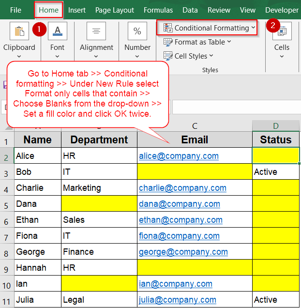
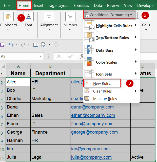
➤ Go to the Home tab >> Click Conditional Formatting >> Choose New Rule.
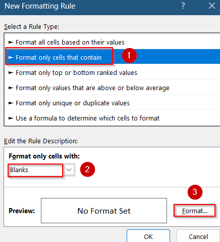
➤ Select Format only cells that contain.
➤ Under “Format only cells with”, choose Blanks from the dropdown.\
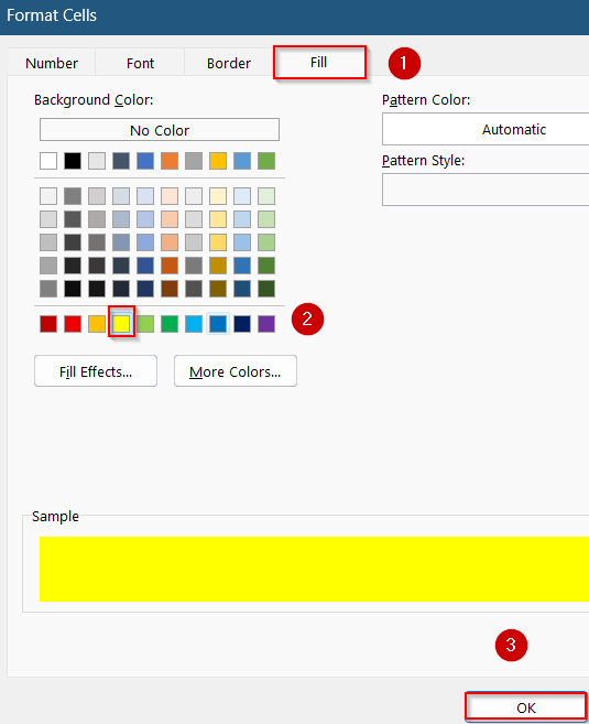
➤ Click Format, pick a fill color (e.g., yellow), and press OK twice to apply the rule.
Use Excel’s Built-in 'Blanks' Option for Conditional formatting
This method uses Excel’s default conditional formatting rule to highlight truly blank cells containing nothing at all. It’s the fastest way to spot empty entries in your data without writing any formulas. However, keep in mind that this option only detects cells that are completely empty. It won’t catch cells that look blank but actually contain formulas returning “” or space characters.
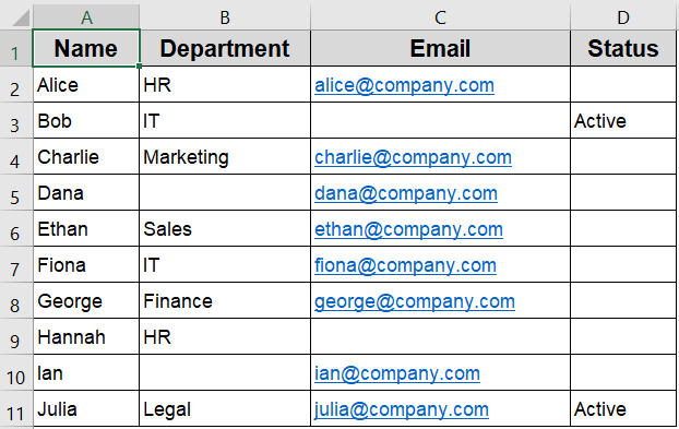
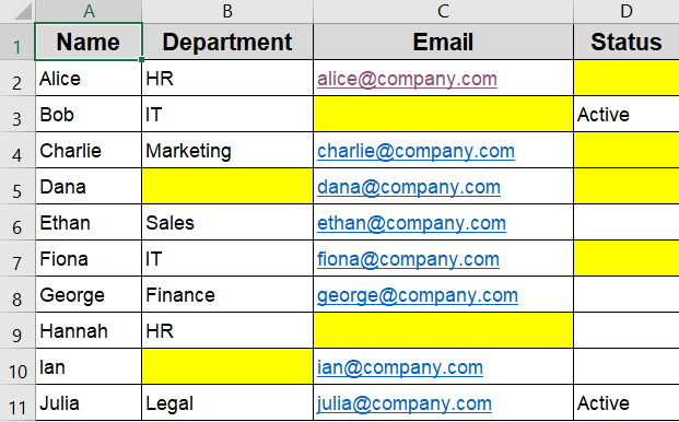
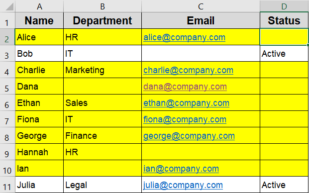
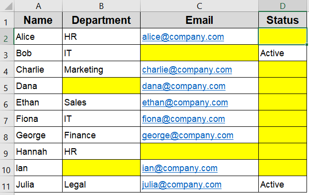
The dataset below includes Name, Department, Email, and Status columns. It contains a mix of true blanks and empty strings (=””), making it perfect for testing different conditional formatting techniques for blank cells.
Steps:
➤ Select the range of cells where you want to find blanks such as A2:D11.
➤ Go to the Home tab >> Click Conditional Formatting >> Choose New Rule.

➤ Select Format only cells that contain.
➤ Under “Format only cells with”, choose Blanks from the dropdown.
➤ Click Format, pick a fill color (e.g., yellow), and press OK twice to apply the rule.
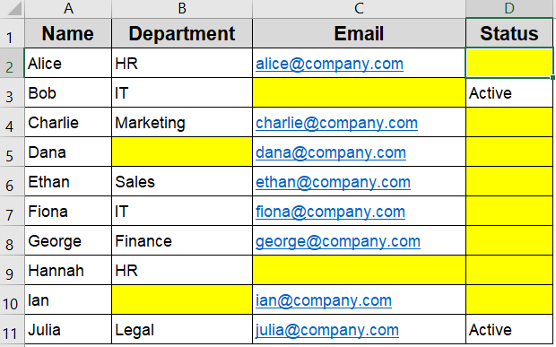
Excel will now highlight all truly and visually empty cells in your selected range.
Use ISBLANK or OR Function in a Custom Formula
This method allows more control by using a custom formula in Excel’s conditional formatting. The ISBLANK function checks whether a cell is truly empty, not even containing a formula or space. However, in cases where cells contain an empty string (“”) or a space character that makes them look blank, you’ll need to use the OR function instead. Together, these formulas help catch both true blanks and blank-looking entries.
Steps:
➤ Select the range of cells where you want to find blanks such as A2:D11.
➤ Go to the Home tab >> Click Conditional Formatting >> Choose New Rule.
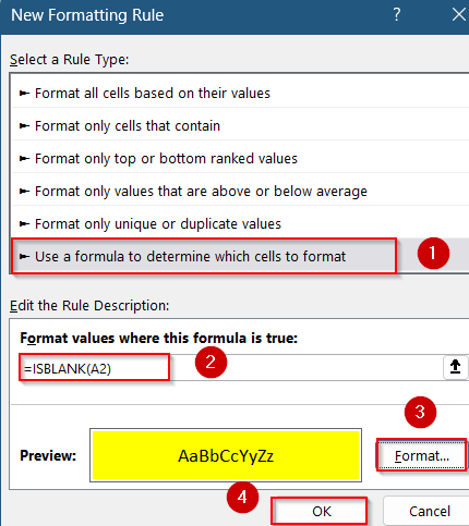
➤ Choose Use a formula to determine which cells to format.
➤ Enter the formula:
=ISBLANK(A2)
➤ Click Format, choose a fill color, and click OK to apply.
Any cell that is completely empty will now be highlighted.
➤ Alternatively, to highlight empty strings as well, use this formula instead:
=OR(A2=””, A2=” “)
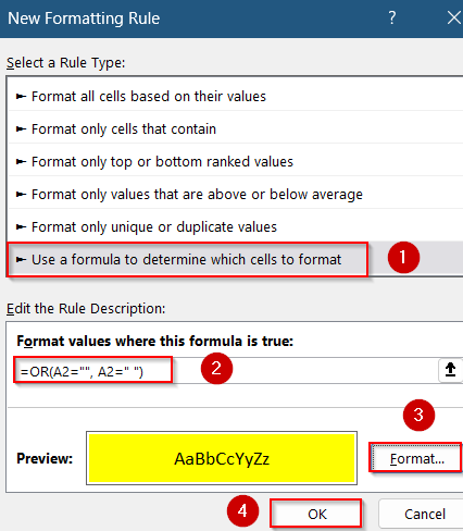
This formula captures cells that visually appear blank but may contain an empty string or a single space, making it more comprehensive than the ISBLANK function alone.

Highlight Blank Cells or Entire Row with a Formula
Sometimes, cells may look blank but actually contain formulas returning an empty string (“”). These aren’t detected by functions like ISBLANK. To handle such cases, you can use a simple formula that checks whether the cell appears empty even if it technically isn’t.
This method is useful when you want to apply conditional formatting to blank cells in a specific column, such as Column D. We can also highlight the entire row for blanks or empty strings.
Steps:
➤ Select the range of cells where you want to find blanks such as A2:D11.
➤ Go to the Home tab >> Click Conditional Formatting >> Choose New Rule.

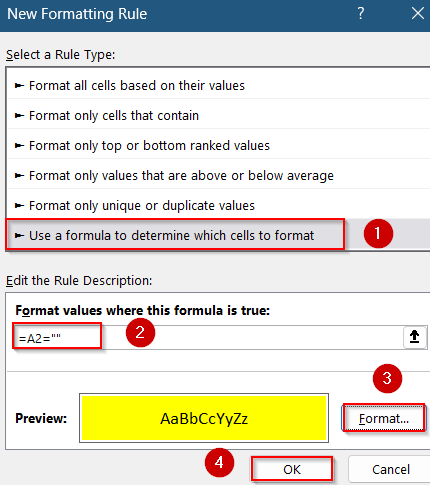
➤ Choose Use a formula to determine which cells to format.
➤ Use the following formula to detect empty-looking cells:
=A2=””
This formula highlights cells that either are blank or contain an empty string.
➤ Click Format, choose a fill color (such as yellow), and click OK to confirm.
➤ Press OK again to apply the rule.
Now all visually and truly blank cells are highlighted.

➤ If you want to check for blanks specifically in column D but highlight the entire row based on that condition, use this formula:
=$D2=””
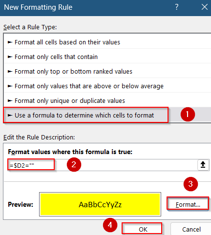
This checks if the cell in column D is visually blank, and applies formatting to every row where that condition is true. It’s especially useful when evaluating data completeness in structured lists.
Use LEN Function to Detect All Visually Blank Cells
The LEN function returns the number of characters in a cell. If that number is zero, the cell is either completely blank or contains an empty string returned by a formula like =””. This method is especially useful when you want to highlight cells that look blank but aren’t caught by the ISBLANK function, including those with hidden formulas.
Steps:
➤ Select the range of cells where you want to find blanks such as A2:D11.
➤ Go to the Home tab >> Click Conditional Formatting >> Choose New Rule.

➤ Choose Use a formula to determine which cells to format.
➤ Type this formula:
=LEN(A2)=0
➤ Click Format, set a fill color, then click OK twice.
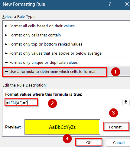
This works well for detecting blanks and formula-driven empty strings.
Frequently Asked Questions
What qualifies as a blank cell in Excel?
A blank cell can be truly empty, contain an empty string from a formula, or even a space character. Excel treats each differently, so detecting all blanks may require specific functions like LEN or OR function.
Why doesn’t ISBLANK highlight cells that appear empty?
ISBLANK function only highlights cells that are completely empty, not those with formulas that return “” or cells with space characters. For visually blank cells, using formula =A2=”” or LEN(A2)=0 gives better coverage.
How can I highlight an entire row based on a blank in one column?
To highlight a row when a specific column is blank, use a formula like =$D2=”” in conditional formatting. Apply it to the entire dataset so the whole row responds to that column’s condition.
What’s the difference between A2=”” and LEN(A2)=0 in conditional formatting?
A2=”” checks if a cell visually appears blank but may miss hidden characters. LEN(A2)=0 is more robust. It detects blanks, empty strings, and formulas that return nothing, giving you more reliable formatting.
Can conditional formatting catch cells with only space characters?
Yes, use OR function in your formula. This captures both truly blank cells and those that appear blank but contain a single space, which can interfere with filtering, sorting, or formulas.
Wrapping Up
In this tutorial, we learned how to apply Conditional Formatting to blank cells using a variety of reliable methods. From built-in options like “Blanks” to custom formulas like ISBLANK, LEN, or OR functions checks, Excel gives you flexibility to catch both visible and actual blanks. Feel free to download the practice file and share your feedback.