Creating a list from a range in Excel is one of the most versatile skills you can master for organizing and analyzing data. Whether you’re building a simple drop-down menu for quick selections, designing a dynamic list that updates automatically when new data is added, or filtering results based on specific conditions, Excel offers multiple approaches to suit your needs. Lists are widely used in reports, dashboards, forms, and data entry sheets to maintain consistency and save time. Depending on your project, you might need a static list that never changes, a list that responds to category selections, or even one that pulls values meeting several criteria.
In this article, we’ll walk through several practical methods starting from basic data validation to advanced formula-based and VBA-generated lists, so you can choose the best technique for your scenario.
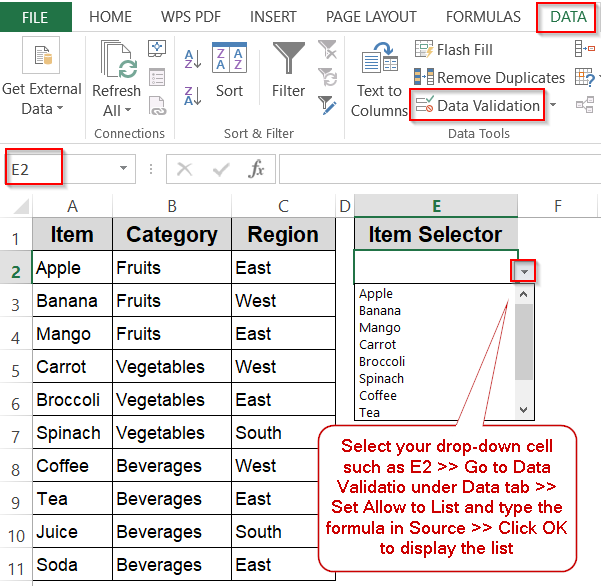
Steps to create a list from a range in Excel:
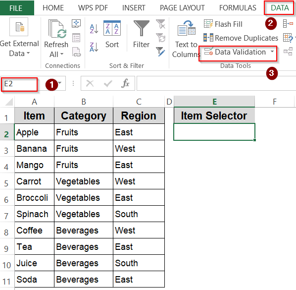
➤ Select the cell where you want the drop-down list such as E2.
➤ Go to Data tab >> Data Validation.
➤ In Allow, select List.
➤ In Source, select your range, for example: =$A$2:$A$11
➤ Click OK. Now, the drop-down will display all products from the Item column for quick and consistent selection.
Creating a Drop-Down List from a Column Range
If you need a quick and straightforward way to make selections from your dataset, creating a basic drop-down list directly from a cell range is the simplest solution. This approach is ideal for cases where your list of items is fixed and doesn’t require advanced filtering or automatic updates. It not only makes data entry faster but also prevents spelling errors and keeps entries consistent across your sheet.
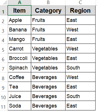
In our sample dataset, the Item column (A2:A11) contains a list of products such as Apple, Banana, and Mango in the Fruits category to Soda in Beverages. By linking this column directly to a drop-down, you’ll be able to select any item from the dataset without manually typing it. This method works well for order forms, survey sheets, or any place where users should only choose from predefined values.
Steps:
➤ Select the cell where you want the drop-down list such as E2.
➤ Go to Data tab >> Data Validation.

➤ In Allow, select List.
➤ In Source, select your range, for example:
=$A$2:$A$11
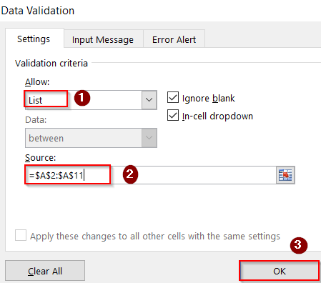
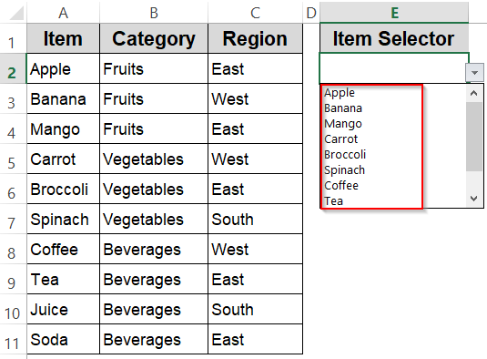
➤ Click OK. Now, the drop-down will display all products from the Item column for quick and consistent selection.
Enable a Dynamic Drop-Down List That Updates Automatically
A dynamic drop-down list is a powerful way to ensure your selection options grow automatically as you add new items to your dataset. Unlike a static list that requires manual updates to include new entries, a dynamic list adapts in real time which saves you time and prevents errors caused by outdated data validation ranges.
Using the sample dataset where your Item list currently spans A2:A11, this method allows your drop-down to expand whenever you add more products below the existing ones. This is especially useful for ongoing projects like inventory tracking, order management, or any situation where your list is expected to change over time.
Steps:
➤ Select the cell where you want the dynamic drop-down list.
➤ Go to the Data tab >> Data Validation.
➤ In the Allow box, choose List.
➤ In the Source box, enter this formula:
=OFFSET($A$2,0,0,COUNTIF($A$2:$A$11,"<>"))
This formula dynamically counts all non-empty cells from A2 down to A11 and adjusts the list length accordingly.
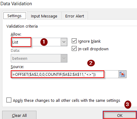
➤ Click OK. Now your drop-down list will automatically include any new items you add within the specified range.

Define a Named Range to Simplify List Management
Using named ranges is a smart way to make your Excel formulas cleaner and easier to maintain. Instead of referencing raw cell addresses every time, you assign a meaningful name to your data range. This approach improves clarity, reduces errors, and makes updates seamless, especially as your dataset grows or changes.
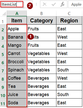
In our example, the Item list from A2:A11 contains a variety of products across categories like Fruits, Vegetables, and Beverages. By naming this range as ItemList, you can quickly reference it anywhere in your workbook, including drop-down lists, without repeatedly selecting the cell range.
Steps:
➤ Highlight the item list range A2:A11 and type ItemList as the name inside the Name Box beside the Formula Bar.
➤ Select the cell where you want the drop-down list.
➤ Open Data Validation, choose List in the Allow box.
➤ In the Source box, type:
=ItemList
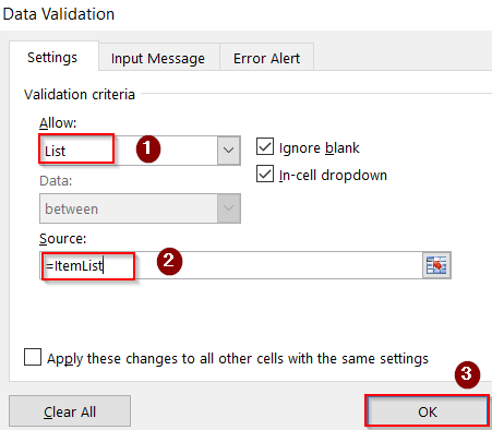
➤ Click OK. Your drop-down now references the named range and will reflect any changes made to ItemList automatically.

Filter a List Based on a Single Criterion
When you want to create a list that dynamically shows items belonging to a specific category, for example, only Fruits, this method uses formulas to filter your dataset based on a single condition. It’s particularly useful when you need drop-down lists or reports that respond to user choices and display only relevant entries.
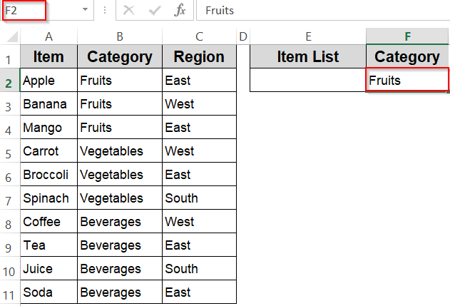
Using the sample dataset, the Category column is in B2:B11, and you can specify the desired category (like “Fruits”) in cell F2. The formula will then extract all matching items from the Item column (A2:A11) that belong to that selected category.
Steps:
➤ Set up your criteria in the F2 cell.
➤ Select the cell where you want your filtered list to start appearing.
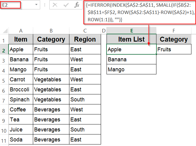
➤ Enter this array formula (for Excel 2019 and earlier, confirm with Ctrl + Shift + Enter):
=IFERROR(INDEX($A$2:$A$11, SMALL(IF($B$2:$B$11=$F$2, ROW($A$2:$A$11)-ROW($A$2)+1), ROW(1:1))), "")
Here, $C$2:$C$11 is the category range, $F$2 contains the category you want to filter by and the formula returns items from $B$2:$B$11 matching that category.
➤ Drag the formula down to list all matching items.
Create a Filtered List Based on Multiple Criteria
When your data needs to be filtered dynamically by more than one condition such as both Category and Region, this method allows you to generate a list that meets all specified criteria. This is especially useful for dashboards, reports, or drop-downs where selections depend on multiple user inputs.
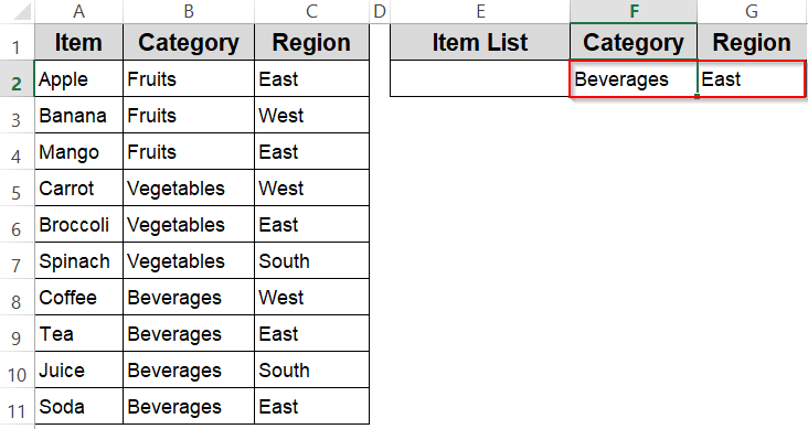
In our sample dataset, the Category column is in B2:B11, and the Region column is in C2:C11. By specifying the desired category in cell F2 and region in cell G2, the formula extracts all items from the Item column (A2:A11) that match both conditions.
Steps:
➤ First set up your criteria in F2:G2.
➤ Select the cell where you want the filtered list to start appearing.
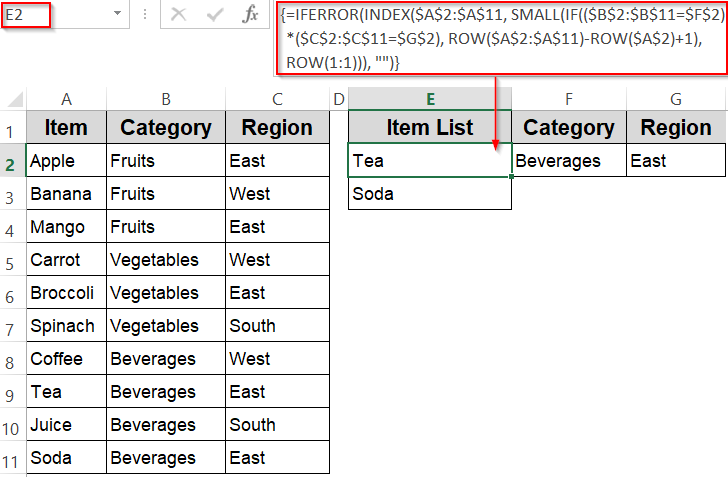
➤ Enter this array formula (press Ctrl + Shift + Enter to confirm in Excel 2019 or earlier):
=IFERROR(INDEX($A$2:$A$11, SMALL(IF(($B$2:$B$11=$F$2)*($C$2:$C$11=$G$2), ROW($A$2:$A$11)-ROW($A$2)+1), ROW(1:1))), "")
Here:$F$2 is the selected category (e.g., Beverages), $G$2 is the selected region (e.g., East) and the formula returns items from $A$2:$A$11 that meet both criteria.
➤ Drag the formula down to display all matching items.
Automate List Creation Using a VBA Macro
For users seeking advanced automation beyond formulas and built-in features, VBA macros offer an efficient way to generate and manipulate lists in Excel. With VBA, you can programmatically extract, copy, or transform data based on custom logic, saving time on repetitive tasks or complex filtering.
In this example, the macro copies the Item list from A2:A11 and pastes it starting at cell E2. This simple script can be easily customized to include filters, sorting, or other automation steps depending on your needs.
Steps:
➤ Press Alt + F11 to open the VBA editor.
➤ Go to Insert >> Module.
➤ Paste the following code:
Sub CreateDropdownInE2()
    With Range("E2").Validation
        .Delete ' Remove existing validation
        .Add Type:=xlValidateList, AlertStyle:=xlValidAlertStop, Operator:= _
            xlBetween, Formula1:="=$A$2:$A$11"
        .IgnoreBlank = True
        .InCellDropdown = True
        .ShowInput = True
        .ShowError = True
    End With
End Sub
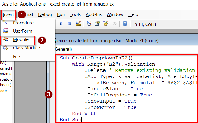
➤ Press F5 key to run the macro and close the VBA editor.
➤ The macro copies the items from A2:A11 and pastes them into the range starting at E2, creating your list automatically.

Frequently Asked Questions
Can I create a drop-down list from multiple ranges?
Yes. Excel allows combining multiple data sources into one list using formulas or named ranges. This is useful when your items are stored in separate locations but need to appear together for user selection.
How do I make my drop-down list update automatically?
A dynamic drop-down can be created using formulas like OFFSET or INDEX with COUNTA, or by converting your range into a table. This ensures newly added items appear instantly without manually changing the validation range.
Why does my formula-based list return errors?
Formula-driven lists can fail due to incorrect range sizes, missing references, or mismatched data. Verifying that all cell references, named ranges, and logic match your dataset structure usually resolves most issues with formula-based lists.
Can I filter my list based on more than one condition?
Yes. Excel supports multi-condition filtering through array formulas, helper columns, or advanced filter tools. These methods allow your list to display only the values meeting all chosen criteria without manually rearranging your original dataset.
Do VBA-based lists work in all Excel versions?
VBA-based drop-downs work in most desktop versions of Excel but aren’t supported in Excel Online. They’re powerful for automation, but require enabling macros and saving the file in a macro-enabled format to function properly.
Wrapping Up
In this tutorial, we explored multiple ways to create a list from a range in Excel starting from simple drop-downs to advanced filtered and dynamic lists. Depending on whether you need a static, filtered, or automatically updating list, these methods give you flexible options for organizing and managing your data. Feel free to download the practice file and share your feedback.