In Excel, highlighting cells based on their values allows you to instantly spot trends, outliers, and important details within your data. Whether you’re dealing with numbers, text, or conditional comparisons, Excel’s built-in Conditional Formatting tools make it easy to emphasize what matters.
In this article, you’ll learn a variety of practical techniques to highlight cells dynamically using simple rules, formulas, logic-based conditions, and Color Scales. From highlighting duplicates to comparing values across columns, these methods will help you bring clarity and focus to your spreadsheets.
Steps to highlight cells in Excel based on value:
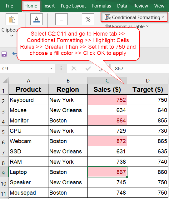
➤ Select the range C2:C11 where your values are stored.
➤ Go to Home >> Conditional Formatting >> Highlight Cells Rules >> Greater Than.
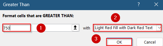
➤ In the dialog box, type a number like 750 as your threshold.
➤ Choose a formatting style (e.g., Light Red Fill with Dark Red Text).
➤ Click OK to apply the rule.
Highlight Values Greater Than a Set Limit
This method highlights cells with values higher than a defined number, making it easy to spot standout figures like top sales or over-limit expenses. For example, if a cell contains 752 and your threshold is 750, it will be highlighted.
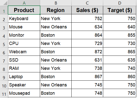
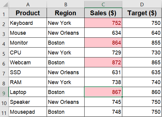
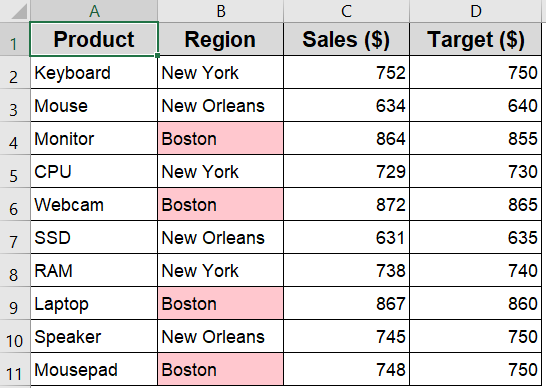
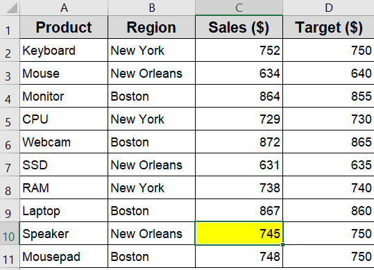
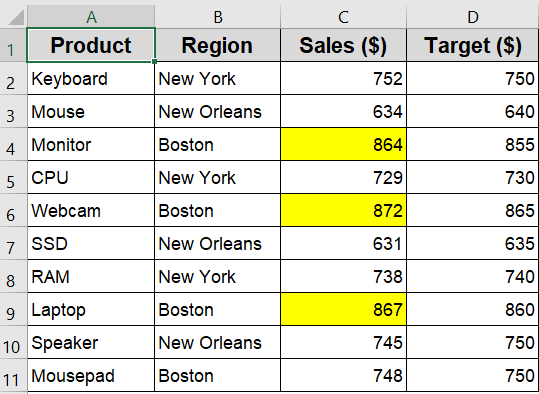
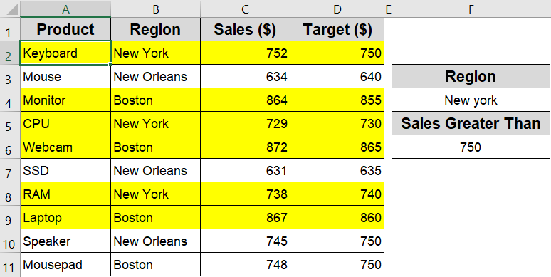
To demonstrate the different highlighting techniques, we’ll use a simple dataset that lists products, their regions, sales figures, and corresponding targets.
Steps:
➤ Select the range C2:C11 where your values are stored.
➤ Go to Home >> Conditional Formatting >> Highlight Cells Rules >> Greater Than.
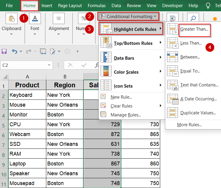
➤ In the dialog box, type a number like 750 as your threshold.
➤ Choose a formatting style (e.g., Light Red Fill with Dark Red Text).
➤ Click OK to apply the rule.
Cells with values above 750 will now stand out visually, helping you focus on key metrics.
Highlight Top N Values
If you want to instantly identify the highest-performing entries in a dataset like the top 3 products with the highest Sales, you can use Excel’s built-in Top/Bottom Rules. This helps you visually pinpoint standout values in a large list. In our dataset, we’ll focus on the Sales column to highlight the 3 top-selling items based on their sales figures.
Steps:
➤ Select the range C2:C11, which contains all the Sales data.
➤ Go to the Home tab, then click Conditional Formatting > Top/Bottom Rules > Top 10 Items.
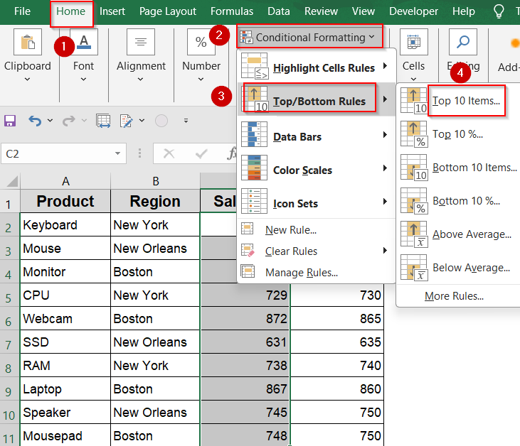
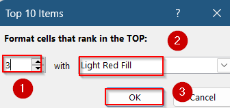
➤ In the dialog box, change the number from 10 to 3 to highlight the top 3 values.
➤ Choose a formatting style (e.g., Light Red Fill) or create a custom format.
➤ Click OK to apply the rule.
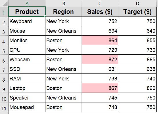
You’ll now see that the three highest sales figures like 872, 867, and 864 are visually emphasized, making them easier to spot in your analysis.
Highlight Duplicate or Unique Values
When working with sales data, it’s helpful to highlight values that occur more than once or only once to detect patterns or data exceptions. For instance, if certain Sales figures are repeated across different products, it might indicate price uniformity or entry errors. Using our dataset, we’ll apply this rule to the Sales column to spot duplicates or unique values.
Steps:
➤ Select the range C2:C11, which includes all the sales values.
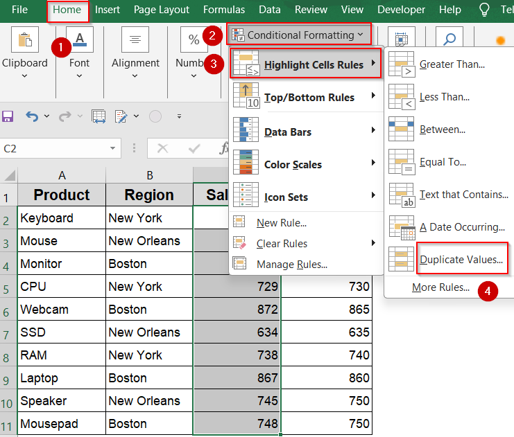
➤ Go to the Home tab, then click Conditional Formatting >> Highlight Cells Rules >> Duplicate Values.
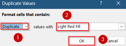
➤ In the pop-up window, choose either Duplicate to highlight repeated values, or Unique to mark one-time entries.
➤ Select a formatting style like colored text or background fill to differentiate the values visually.
➤ Click OK to apply the rule.
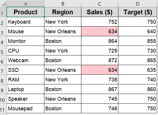
Now, Excel will highlight all duplicate sales figures such as any value that appears more than once or highlight only the unique entries, depending on your selection.
Highlight Based on Text Values
If you want to instantly locate products from a specific region such as Boston you can use a text-based conditional formatting rule. This is especially useful when working with location-based data, like in our dataset’s Region column, where multiple cities appear. This method helps you visually isolate entries tied to a particular area.
Steps:
➤ Select the range B2:B11, which contains all the region names.
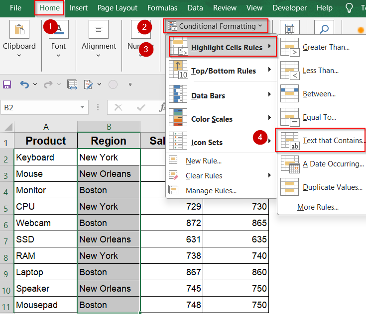
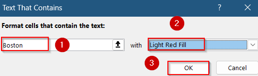
➤ Navigate to the Home tab, then click Conditional Formatting >> Highlight Cells Rules >> Text That Contains.
➤ In the input box, type Boston exactly as it appears in the cells.
➤ Choose a formatting style (e.g., a light green fill or custom font color).
➤ Click OK to apply the rule.
Now, all entries from Boston like Monitor, Webcam, Laptop, and Mousepad will be highlighted, making it easier to filter or analyze region-specific data visually.
Highlight Based on Another Cell’s Value
To perform a comparison between columns such as checking if actual Sales values exceed their corresponding Target value, you can use a formula-based conditional formatting rule. This method is great for performance tracking. In our dataset, we’ll compare values from the Sales column against the Target column to highlight only those entries where the sales surpassed the target.
Steps:
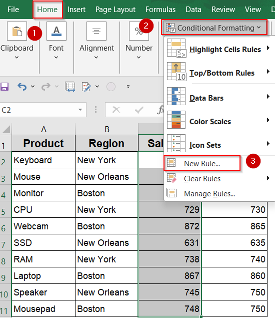
➤ Select the range C2:C11, which contains all sales figures to be evaluated.
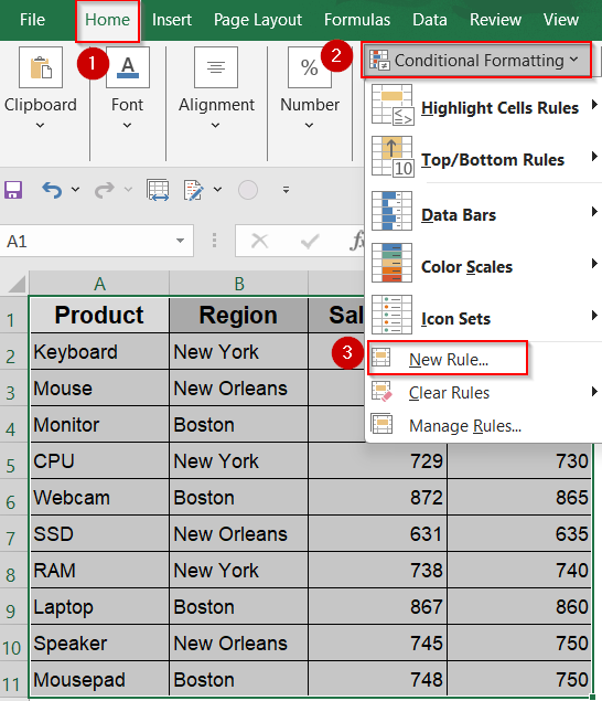
➤ Go to the Home tab, then click Conditional Formatting >> New Rule.
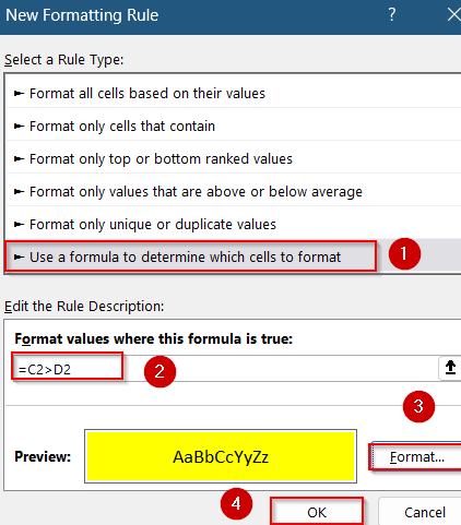
➤ In the New Formatting Rule dialog, select Use a formula to determine which cells to format.

➤ Enter the formula:
=C2>D2
This checks if the value in the Sales column is greater than the corresponding value in the Target column.
➤ Click Format, choose a fill color (e.g., yellow fill for exceeded targets), and press OK.
➤ Confirm again by clicking OK to apply the rule.
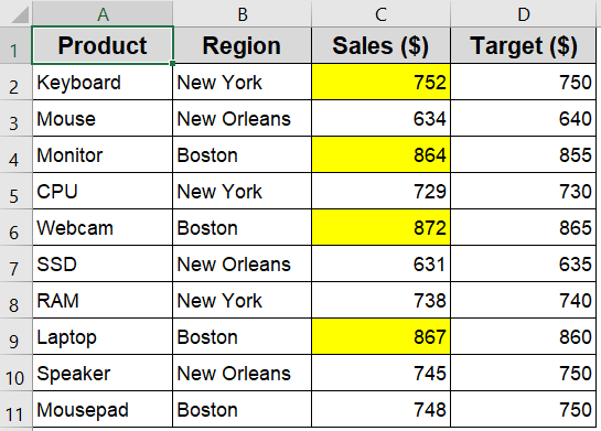
With this rule in place, Excel will highlight all sales entries that outperformed their targets, for example, Keyboard (752 > 750), Monitor (864 > 855), and Webcam (872 > 865).
Highlight Based on Exact Match
When analyzing data, sometimes you need to single out a specific value, for instance, finding the exact Sales figure of 745 to verify pricing, detect anomalies, or flag key entries. This method uses a formula-based rule to highlight cells in the Sales column that match a specified value exactly.
Steps:
➤ Select the range C2:C11, which contains the sales values you want to examine.
➤ Go to the Home tab, then click Conditional Formatting >> New Rule.

➤ Choose Use a formula to determine which cells to format.
➤ Enter this formula:
=C2=745
This checks whether the cell’s value is exactly 745.
➤ Click Format, then choose your desired Fill color (e.g., yellow).
➤ Press OK, and then click OK again to apply the rule.
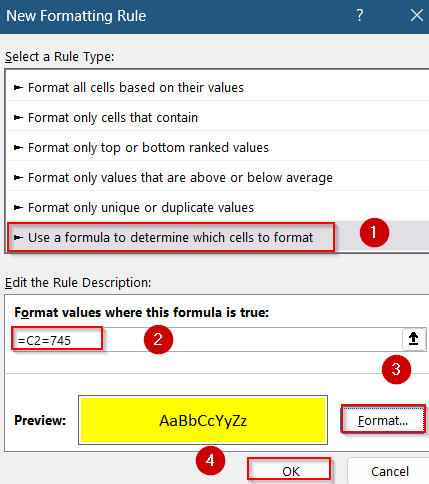
The rule will now highlight any sales entry that equals 745 such as the Speaker sold in New Orleans, so it stands out clearly in your dataset.
Highlight Greater Than Column Average
Highlighting values above the column average helps you quickly spot top performers or outliers in a sales dataset. Instead of manually calculating averages, this method uses a dynamic formula that compares each value in the Sales column against the overall average of that column. It’s especially useful for identifying which products performed better than average without sorting the data.
Steps:
➤ Select the range C2:C11, which includes all sales figures.
➤ Go to the Home tab, then click Conditional Formatting >> New Rule.
➤ Choose Use a formula to determine which cells to format.
➤ Enter this formula:
=C2>AVERAGE($C$2:$C$11)
This checks if each sales figure is greater than the average of the entire column.
➤ Click Format, then choose a fill color or font style that clearly distinguishes the above-average cells.
➤ Click OK twice to apply the rule.
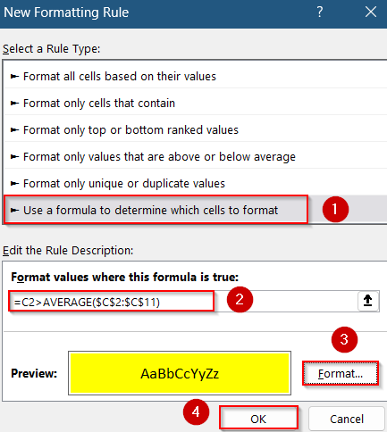
Now, Excel will automatically highlight all sales entries that are higher than the average.
Use AND/OR Logic to Highlight with Multiple Conditions
Sometimes, you need to highlight rows based on multiple conditions such as flagging only those sales from New York that also exceeded a threshold, or highlighting if either condition is met. This method lets you combine logical tests using AND or OR formulas in Excel’s conditional formatting. In our dataset, we’ll evaluate both the Region column (B2:B11) and the Sales column to apply flexible, rule-based highlights.
Steps:
➤ Select the entire range from row 2 to 11 (i.e., A2:D11) so that full rows can be formatted.
➤ Go to the Home tab, then click Conditional Formatting >> New Rule.
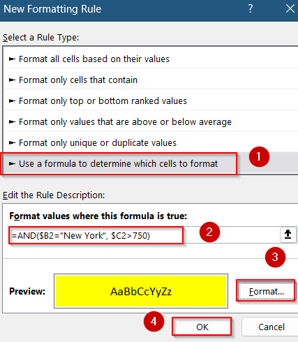
➤ Select Use a formula to determine which cells to format.
➤ To highlight only if both conditions are true (Region is New York AND Sales > 750):
=AND($B2=”New York”, $C2>750)
➤ Click Format, then set your preferred highlighting style (e.g., bold text or a color fill).
➤ Click OK, and again OK to apply the rule.
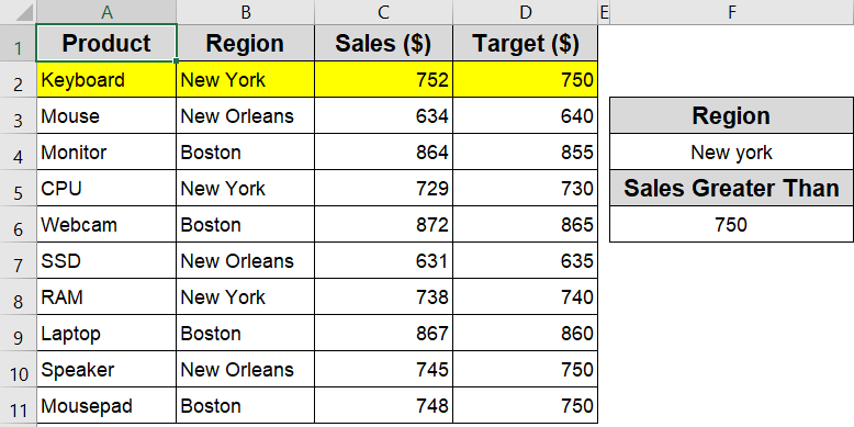
Now, only the row for Keyboard sold in New York will be highlighted.
➤ To highlight if either condition is true (Region is New York OR Sales > 750), use this formula:
=OR($B2=”New York”, $C2>750)
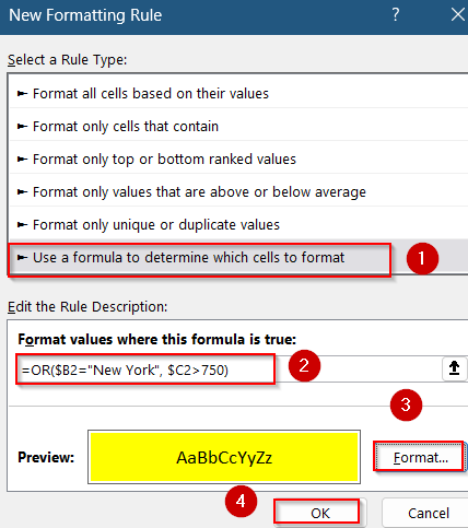
Now the OR formula, multiple rows like Keyboard, Monitor, Webcam, Laptop, and others will be highlighted.
Use Color Scales to Visually Compare Values
If you want to see how all values in a column rank from lowest to highest without setting specific limits, Color Scales is an ideal choice. It applies a gradient of colors to cells, helping you instantly visualize patterns like which products are low, medium, or high performers. In our dataset, applying a color scale to the Sales column provides a heatmap-style view of performance at a glance.
Steps:
➤ Select the range C2:C11, which contains your sales data.
➤ Go to the Home tab, then click Conditional Formatting >> Color Scales.
➤ Choose a preset color scale, for example, Green–Yellow–Red, where green highlights the highest values and red the lowest.
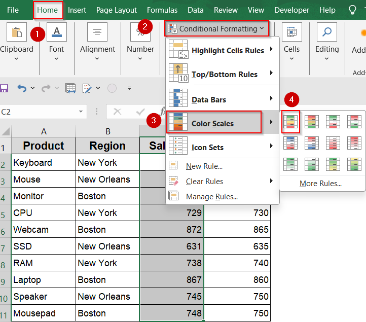
Now Excel will automatically assign colors based on the range of values in the column.
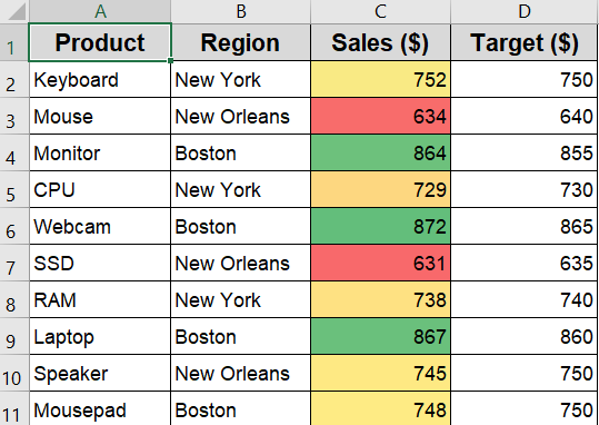
Once applied, the darkest green cell will represent the highest sale (872), while the darkest red will show the lowest sale (631). This method is perfect for spotting trends, outliers, or overall distribution without digging through numbers.
Frequently Asked Questions
Can I highlight cells based on a formula instead of preset rules?
Yes, Excel allows you to create custom rules using formulas in Conditional Formatting. This gives you more flexibility like comparing values across columns or applying logic-based conditions using functions like AND, OR, or AVERAGE.
How do I highlight cells greater than a certain number?
Select your data range, go to Conditional Formatting >> Highlight Cells Rules >> Greater Than, and enter your threshold value. Excel will then highlight all cells that exceed that number using your chosen formatting style.
Is it possible to highlight entire rows based on a single cell’s value?
Yes. You can use a formula with a relative reference (like $C2>50) applied across multiple columns. Just make sure to select the entire row range before applying the conditional formatting rule so that all columns respond to that condition.
Can I highlight text values, like specific regions or product names?
Yes, using Text That Contains under Conditional Formatting lets you highlight cells based on specific words or phrases. It’s useful when filtering by location, product name, or category without using filters or formulas.
Will conditional formatting update automatically if the values change?
Yes, conditional formatting in Excel is dynamic. If the cell values change due to manual edits or formulas, the formatting will automatically update in real time, reflecting the current data and meeting the original condition set.
Wrapping Up
In this tutorial, we explored several effective ways to demonstrate how to highlight cells in Excel based on value. You learned how to highlight cells that are greater than a certain number, above the column average, equal to a specific value, or even those that meet multiple conditions using AND/OR logic. We also covered text-based rules, duplicate detection, and comparing values across columns. Feel free to download the practice file and share your feedback.