

When working with spreadsheets, it’s common to have a mix of text, numbers, and blank cells. Sometimes, you need to visually emphasize entire rows where certain cells contain text, such as product codes, status labels, or remarks. Excel’s Conditional Formatting makes this easy, allowing you to apply custom rules to highlight rows dynamically.
In this article, we’ll explore multiple methods to highlight rows containing text values only, ignoring blank cells and numbers, ensuring your spreadsheet is easy to read and analyze. Let’s get started.
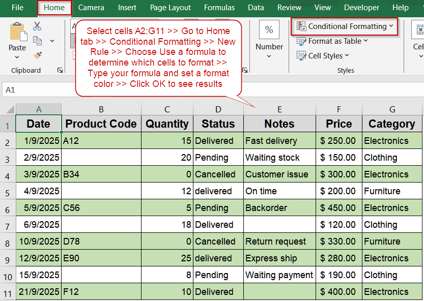
Steps to highlight row if a cell contains any text in Excel:
➤ Select your entire data range (for example, A2:G11).
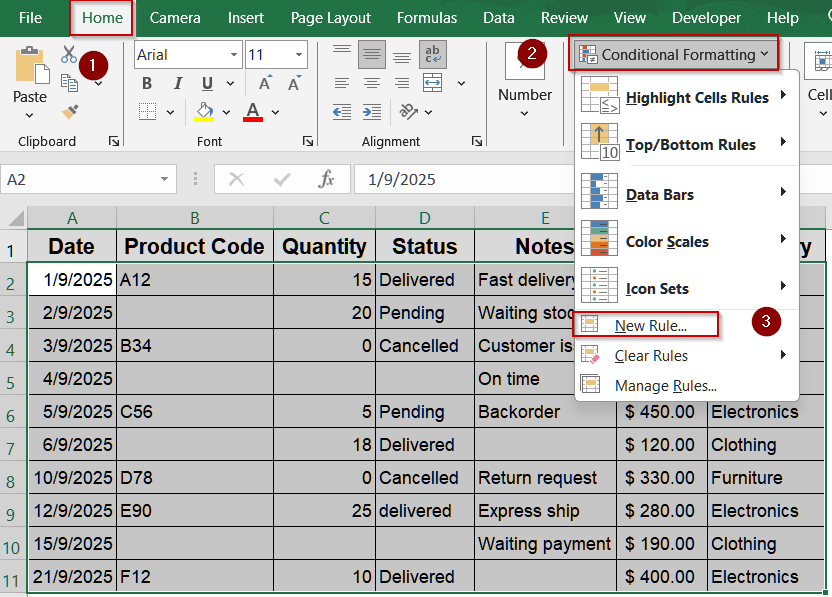
➤ Go to Home >> Conditional Formatting >> New Rule.
➤ Choose Use a formula to determine which cells to format.
➤ Enter the formula below to detect non-empty text cells in column B:
=NOT(ISBLANK($B2))
➤ Click Format, choose your desired fill color, and click OK.
➤ Click OK again to confirm the rule.
Insert a Simple Formula to Highlight Rows Containing Text
This method is the easiest way to identify rows that contain text within a specific column. By combining the ISBLANK and NOT functions, you can tell Excel to ignore empty and numeric cells while highlighting rows that contain any kind of text entry. This approach is perfect for smaller datasets or situations where a single column determines whether a row should stand out.
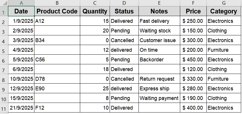
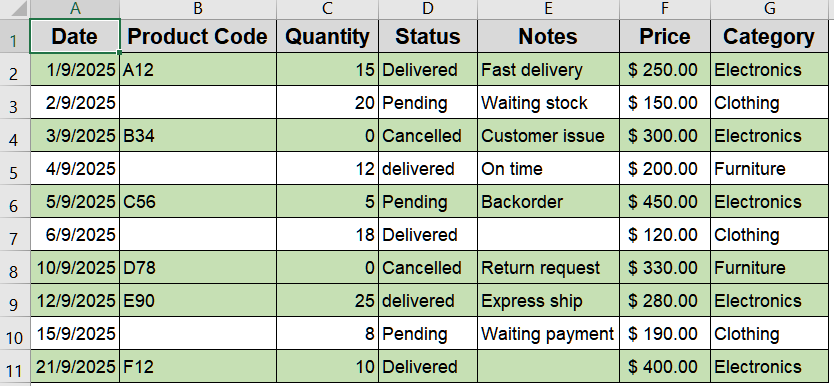
We’ll use the following dataset where product orders with details like codes, quantity, status, notes, and price are recorded. Some cells contain text (e.g., “Delivered”), while others are blank or numeric which is perfect for demonstrating how to highlight rows containing text:
Steps:
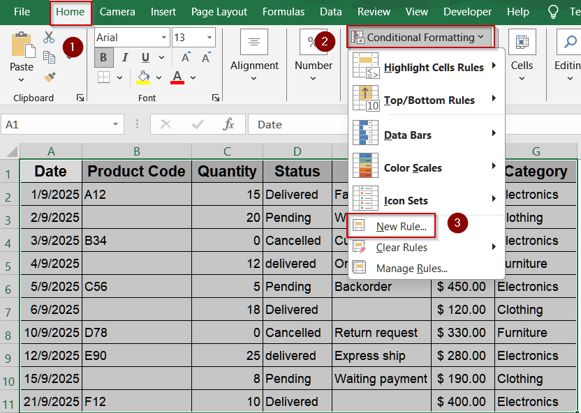
➤ Select your entire data range (for example, A2:G11).
➤ Go to Home >> Conditional Formatting >> New Rule.
➤ Choose Use a formula to determine which cells to format.
➤ Enter the formula below to detect non-empty text cells in column B:
=NOT(ISBLANK($B2))
➤ Click Format, choose your desired fill color, and click OK.
➤ Click OK again to confirm the rule.
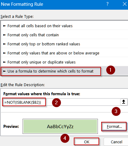
Rows with text in column B will now be highlighted automatically.
Identify Specific Words Using the SEARCH Function
If you want to highlight rows containing a particular keyword or phrase, the SEARCH function is an ideal tool. It can search across multiple columns by combining them into one logical string, and it’s not case-sensitive, making it versatile for tracking key text patterns like “Delivered” or “Pending.”
Steps:
➤ Highlight your data range.
➤ Go to Home >> Conditional Formatting >> New Rule >> Use a formula.
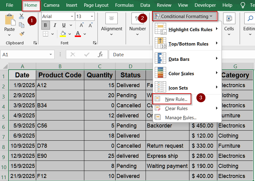
➤ Type the following formula to find the word “Delivered” in columns B to D:
=ISNUMBER(SEARCH("Delivered",$B2&$C2&$D2))
➤ Click Format, choose a color, and click OK.
➤ Confirm by clicking OK again.
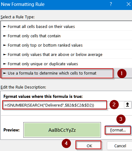
Rows containing “Delivered” in any of these columns will now be automatically highlighted.
Case-Sensitive Row Highlighting Using FIND Function
If it’s important to distinguish between uppercase and lowercase text (like “Delivered” and “delivered”), the FIND function gives you precise control. Unlike SEARCH, FIND function only highlights rows that match your text exactly as typed, making it suitable for detailed or sensitive data reviews.
Steps:
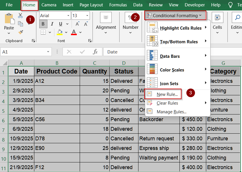
➤ Select your entire range of data.
➤ Go to Home >> Conditional Formatting >> New Rule >> Use a formula.
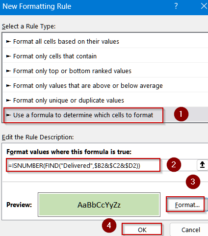
➤ Enter this formula:
=ISNUMBER(FIND("Delivered",$B2&$C2&$D2))
➤ Choose a fill color from the Format menu and click OK.
➤ Apply the rule by clicking OK once more.
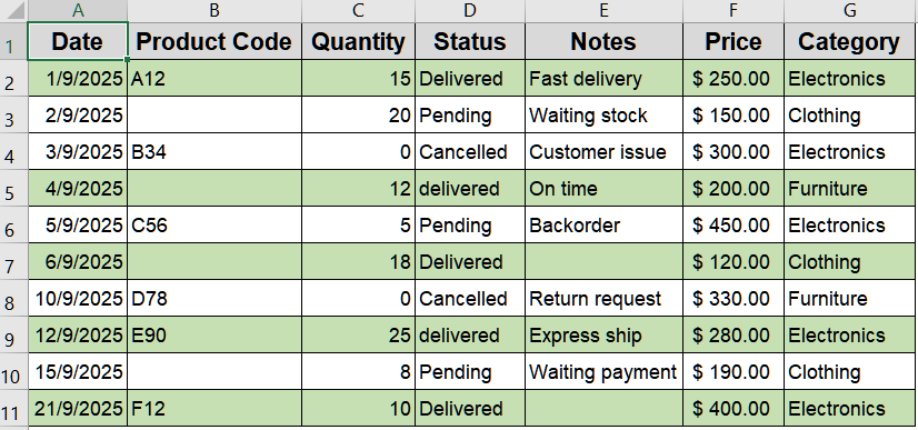
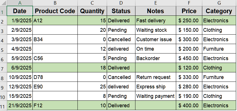
Only rows containing the exact case-specific word “Delivered” will be highlighted.
Highlight Rows Based on Multiple Conditions Using AND Function
Sometimes, you may need to highlight a row only when multiple conditions are met such as when a cell contains text and another cell contains a numeric value above a certain threshold. The AND function makes it possible to apply both rules simultaneously for precise conditional formatting.
Steps:
➤ Select your dataset range.
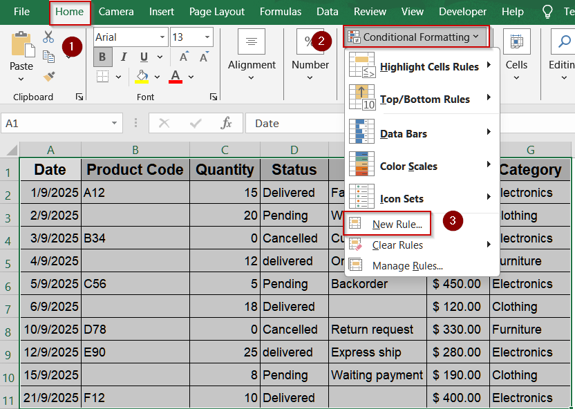
➤ Navigate to Home >> Conditional Formatting >> New Rule >> Use a formula.
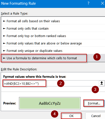
➤ Use this formula to check that column B contains text and column C’s value is greater than 10:
=AND($C2>10,$B2<>"")
➤ Click Format, choose your highlight color, and click OK.
➤ Apply the rule with OK.
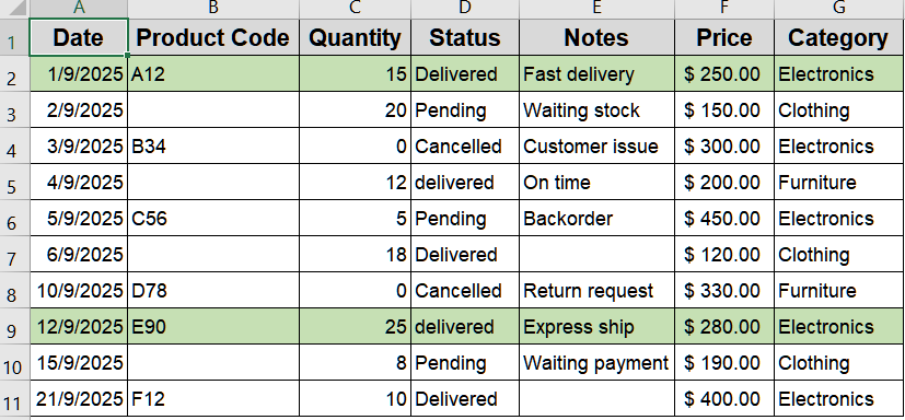
Excel will now highlight rows that satisfy both text and numeric conditions.
Highlight Rows Using OR Logic Across Columns
If your text could appear in any of several columns, OR logic helps ensure no potential match is missed. This method highlights rows where at least one of multiple columns contains text, making it a great fit for datasets with varied data entry points.
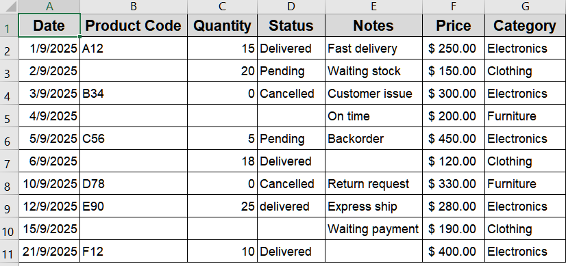
We’ll use the following modified dataset for demonstration:
Steps:
➤ Select your full data range.
➤ Go to Home >> Conditional Formatting >> New Rule >> Use a formula.
➤ Enter this formula:
=OR($B2<>"",$C2<>"",$D2<>"")
➤ Choose your preferred fill color and click OK.
➤ Press OK again to apply.
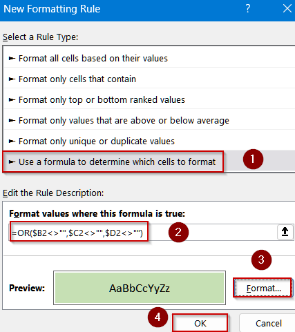
Now, any row with text in columns B, C, or D will be instantly highlighted.
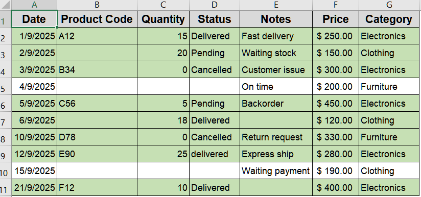
Detect Text Across Multiple Columns Using MATCH Function
When your dataset has multiple columns where text might appear, the MATCH function can quickly identify and highlight any row containing text in any of those columns. It’s an excellent method for spreadsheets with mixed data types where text entries can appear anywhere.
Steps:
➤ Select your data range (e.g., A2:G11).
➤ Go to Home >> Conditional Formatting >> New Rule >> Use a formula.
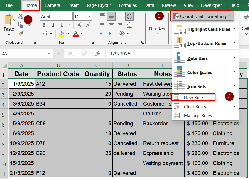
➤ Enter this formula to scan columns B through D for text:
=ISNUMBER(MATCH("*",$B2:$D2,0))
➤ Click Format, pick a highlight color, and click OK.
➤ Press OK again to apply the rule.
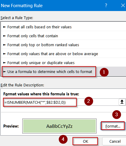
All rows that contain any text within columns B, C, or D will now be highlighted.
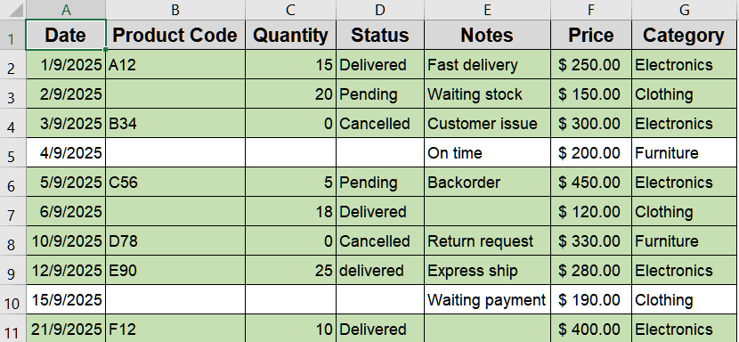
Use a Drop-Down Selection to Control Row Highlighting
For interactive and dynamic data management, you can link conditional formatting to a drop-down list. When you select a specific value from the list, all rows containing that same value will automatically highlight, making filtering and visual sorting easy.
Steps:
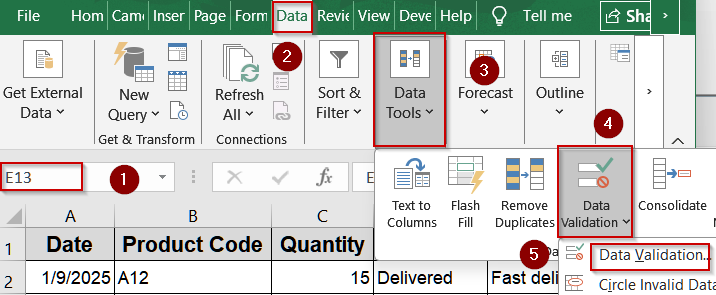
➤ Select cell E13 and go to Data >> Data Validation under Data Tools.
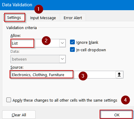
➤ From the Settings tab, set Allow to List.
➤ Type the following formula in the source box:
Electronics, Clothing, Furniture
➤ Hit OK to see the drop-down.
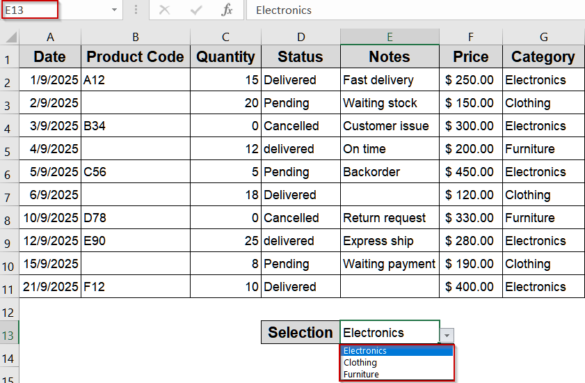
➤ Select your data range.
➤ Go to Home >> Conditional Formatting >> New Rule >> Use a formula.
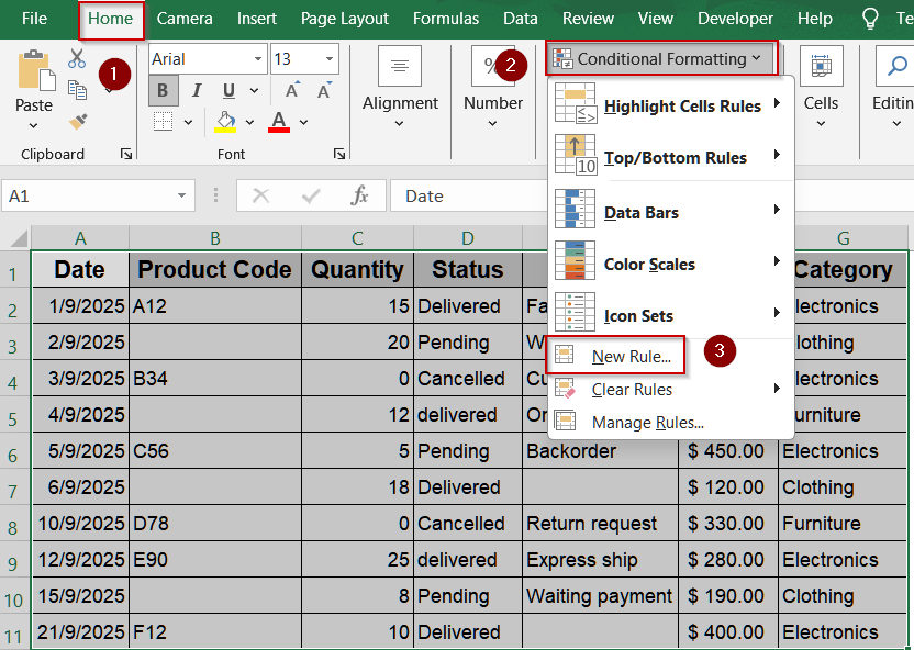
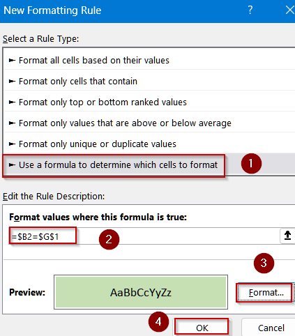
➤ Type the following formula:
=$G2=$E$13
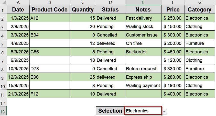
Here, $E$13 is the cell containing your drop-down selection.
➤ Click Format, pick a fill color, and press OK.
➤ Apply the rule by clicking OK again.
Rows that match the selected drop-down value will now be highlighted dynamically.
Downloadable Resources
Get our practice workbook or necessary files that we have worked with to prepare this article.
Highlight Row If Cell Contains Any Text.xlsx
Frequently Asked Questions
Can I highlight rows containing text in multiple columns at once?
Yes, using conditional formatting with formulas like OR or MATCH, you can check multiple columns in a row. Any row containing text in the specified columns will be highlighted automatically, making it easy to track important data.
Will this method work if the row contains numbers along with text?
Yes, the formulas can be designed to highlight only rows where at least one cell contains text. Numbers alone won’t trigger formatting, ensuring your spreadsheet highlights only meaningful textual data.
Can I make the text highlight case-sensitive?
Yes. Using the FIND function in your conditional formatting formula allows case-sensitive detection. This ensures that only cells with exact text matching the case you specify will trigger row highlighting.
Can I highlight rows dynamically based on a drop-down selection?
Yes. By linking conditional formatting formulas to a drop-down cell, you can automatically highlight rows that match the selected value. This makes filtering and visual tracking of specific entries much easier.
Is it possible to combine multiple conditions for highlighting rows?
Yes. You can use the AND or OR functions within conditional formatting formulas to combine conditions, such as text in a column plus numeric thresholds, providing full control over which rows are highlighted.
Wrapping Up
In this tutorial, we explored multiple ways to highlight rows in Excel if a cell contains text. Using conditional formatting with formulas like ISBLANK, SEARCH, MATCH, and AND, you can easily emphasize rows containing meaningful text, ignore numbers, and improve spreadsheet readability. Feel free to download the practice file and share your feedback.