
When we work with the before and after data of the same observations, we often need to compare the results of the two groups to identify any changes. For this, we can compare the means of these two groups. However, a simple comparison is not enough to conclude that the change happened due to any factor applied to the after-dataset. To overcome it, we need to conduct a paired t-test to support our findings statistically.
Suppose you are working with an obese patient’s dietary plan to lose weight. You took the records of their weights before following the dietary plan. Then you record their weight after following the plan for one month. Now you need to compare the before and after results to determine if the dietary plan helped the patients lose weight. In such a case, you can do a paired t-test to identify any statistically significant change.
In this article, we will explain two different methods, including using the T.TEST function and the built-in Data Analysis ToolPak, to conduct a paired t-test in Excel.
➤ First, click on cell D1 and write Paired T Test. You can choose any empty cell.
➤ Now, select cell D2 and insert the following formula:
=T.TEST(B2:B11, C2:C11, 2, 1)
Here,
B2:B11 is the range of the before data.
C2:C11 is the range of after data.
2 indicates it is a two-tailed paired t-test. That is, the effect seen in the after data can be both negative and positive.
1 specifies that the test is a paired t-test.
➤ Press Enter, and you will see the p-value of the t-test.

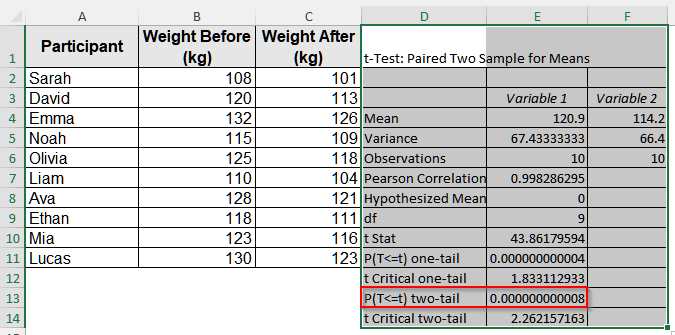
Here, the p-value is less than 0.01. That is, the result is highly significant. So, the dietary program has a significant effect on weight loss.
Do a Paired T Test With the T.TEST Function in Excel
If you want to get a direct p-value for your paired t-test and come to a decision, the T.TEST function is the best choice. It returns the p-value directly in the cell.
We will use the dataset below to explain how you can conduct a paired t-test in Excel with the T.TEST function.

This is a dataset of participants of a weight loss program where the before weight is their initial weight, and the after weight is the weight after following the dietary plan for two months.
Steps:
➤ First, click on cell D1 and write Paired T Test. You can choose any empty cell.
➤ Now, select cell D2 and insert the following formula:
=T.TEST(B2:B11, C2:C11, 2, 1)
Here,
B2:B11 is the range of the before data.
C2:C11 is the range of after data.
2 indicates it is a two-tailed paired t-test. That is, the effect seen in the after data can be both negative and positive.
1 specifies that the test is a paired t-test.
➤ Press Enter, and you will see the p-value of the t-test.

Here, the p-value is less than 0.01. That is, the result is highly significant. So, the dietary program has a significant effect on weight loss.
Use the Data Analysis ToolPak to Perform a Paired T Test
The Data Analysis ToolPak gives a detailed report on a paired t-test. So, if you want to see other statistical features like mean, variance, degrees of freedom, etc., then this built-in Excel feature is the best choice. Also, with this tool, you do not need to write any code.
Steps:
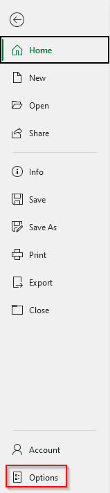
➤ First, enable the Data Analysis ToolPak. Open your Excel dataset and go to the File tab on the upper menu bar.

➤ You will see a new window. Select the Options in it.
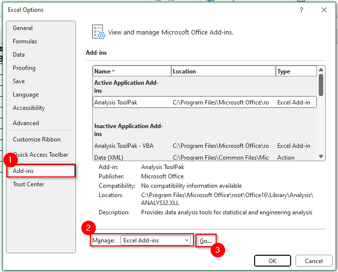
➤ Then, a new page will appear. On that page, click on Add-in. Then, at the bottom, in the Manage box, select Excel Add-ins and then click on Go.
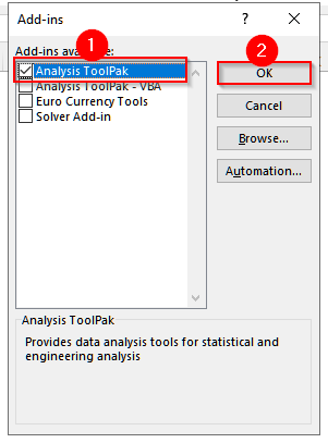
➤ You will see a new pop-up. Check the box for Analysis ToolPak on it, and then click OK.
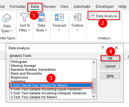
➤ Go to the Data tab from the upper ribbon. Then, select the Data Analysis option.
➤ Another pop-up will appear. Select t-Test: Paired Two Sample for Means, then click OK.
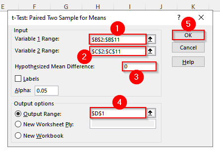
➤ Now, you will see a pop-up asking to specify the ranges. In the Variable 1 Range, select the before data range, i.e., B2:B11, and in the Variable 2 Range, select the range for after data, i.e., C2:C11.
➤ In the Hypothesized Mean Difference box, enter 0.
➤ Finally, in the Output Range, select D1 and click on OK.
➤ Now, the result for this paired t-test will appear beside your dataset.
Frequently Asked Questions
When Should I Use a Paired Sample T Test Instead Of an Independent Sample T Test?
If your dataset has two groups and each observation of one group is directly linked to an observation of another group, you need to do the paired sample t-test. Because in such a dataset, the observations of two groups act as a pair. Usually, all before-and-after dataset requires a paired sample t-test.
Do I Need to Arrange the Data in Pairs before Doing a Paired T-Test in Excel?
Yes, you need to arrange your dataset in pairs before doing a paired t-test in Excel. Because in a paired t-test, each observation in one group must correspond directly to an observation in the other group, and Excel uses the row position to determine these pairs. So, if the data are misaligned, the results will be incorrect.
How Can I Arrange a Dataset into Pairs in Excel Before Doing the Paired T-Test?
You can arrange the pairs manually or using a formula. Usually, this type of data has a unique identifier for each observation. For each identifier, place one observation in a cell and the other observation beside it, like before and after data for one identifier are side by side in a row. You can also use the VLOOKUP or INDEX-MATCH functions to arrange the pairs.
Wrapping Up
In this article, we have learned two different methods to conduct a paired t-test in Excel. Use the T.TEST function if you are in a rush and want to see the p-value only. And, if you want to see other statistical features, including mean, degrees of freedom, etc, and do not want to write a formula, use the Data Analysis Toolpak. Reach out if you have any inquiries or want to share any feedback.