

Rounding numbers in Excel is often necessary for improving data readability and consistency, especially when working with large numerical values like measurements, financial figures or statistical results. While formulas like ROUND, ROUNDUP, and ROUNDDOWN can be used to round numbers in Excel, we can also round numbers using Excel’s built-in number formatting tools, without needing to write any formulas. There is one difference worth knowing before you start: formatting changes only how a number is displayed, while the full value stays in the cell and is what any later calculation uses. Of the four methods below, only Power Query actually rewrites the stored value. If you would rather use a formula after all, start with how to round up a formula result in Excel.
To round numbers in Excel without using any formula, follow the steps below:
➤ In your spreadsheet file, select the header of the column whose value you want to round.
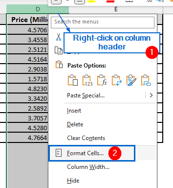
➤ Next, right-click on the column header and select Format Cells from the context menu.
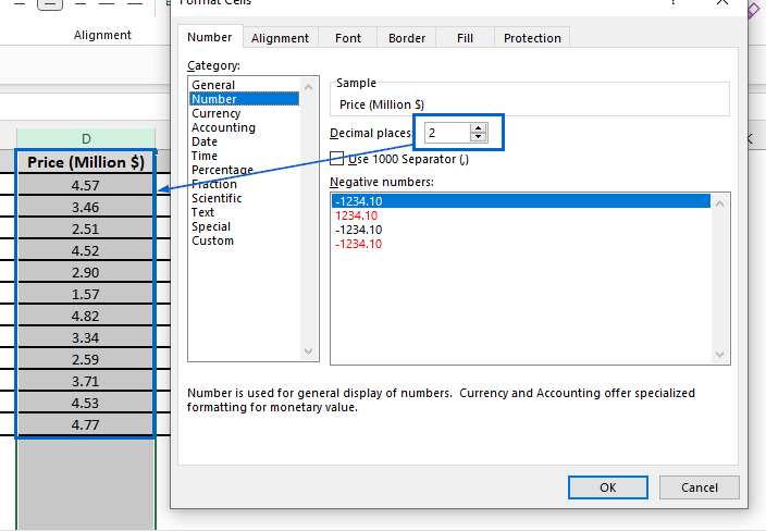
➤ From the Category list, choose Number.
➤ In the Decimal places box, enter the number of decimal places to which you want to round your values, then click OK.
In this article, we will learn 4 effective methods by using which you can easily round numbers in Excel without using any formula.
Use Format Cells to Round Numbers
This is the most effective and efficient way of rounding numbers in Excel without using formulas. Format Cells is a powerful feature that allows users to customize the way data is displayed without changing the actual values.
In the sample dataset, we have a worksheet called “Real Estate Listings” containing information about Property ID, City, Type, Price (Million $) and Name of the person listed by. By using the Format Cells feature, we will round the decimal values in Column D to two decimal places and display the results in the “Format Cells” worksheet. The same dialogue also handles rounding to a larger scale. Choose Custom instead of Number and put a comma at the end of the format code: #,##0, displays each value in thousands, so 1,234,567 shows as 1,235. Each additional comma divides the display by another thousand. As with every other formatting route, the underlying value is unchanged – the cell still holds 1,234,567 for any formula that reads it. If it is meaningful digits you need to control rather than decimal places, see how to change significant figures.
Steps:
➤ Head to the Format Cells worksheet, right-click the header of Column D to open the context menu, then select Format Cells.
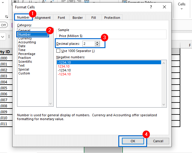
➤ In the Format Cells dialogue box, click on Number from the category list. Then, enter “2” in the Decimal places box and click OK.
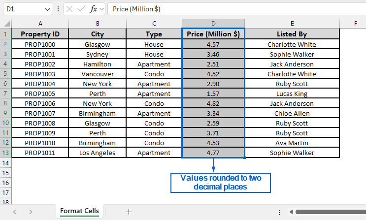
➤ Column D is now formatted to display numbers rounded to two decimal places.
Use the Decrease Decimal Button to Adjust Decimal Places
This is another useful technique that utilizes Decrease Decimal button from the Number group to round off values in Excel. Using the same dataset, we’ll apply this method to round the values in Column D to two decimal places. The updated dataset will be stored in a separate worksheet called “Decrease Decimal Button”.
Steps:
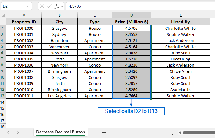
➤ In the Decrease Decimal Button worksheet, select cells D2 to D13.
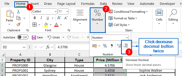
➤ Next, go to the Home tab and from the Number group, click on the Decrease Decimal button. Each click removes one displayed decimal place, so the number of clicks depends on how many decimals your column shows to begin with. This dataset displays four, so click twice to reach two decimal places.
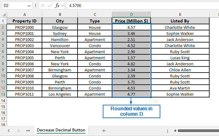
➤ All values in column D should now be rounded to 2 decimal places.
Use Number Format Dropdown for Quick Two-Decimal-Place Rounding
The Number Format dropdown in Excel allows users to quickly apply a predefined set of number formats to their data. Unlike other methods, this method automatically rounds values to two decimal places by default, without requiring you to enter any specific decimal setting. We will again work with the same dataset and, by using the Number Format dropdown, round values in column D to two decimal places. We will display the modified dataset in a separate “Number Format” worksheet.
Steps:
➤ Head to the Number Format worksheet and select cells D2 to D13.
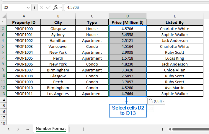
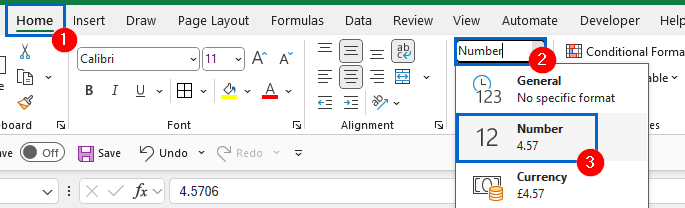
➤ Next, head to the Home tab and from the Number Format dropdown, choose Number option.
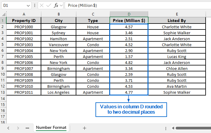
➤ You should now see your values in column D rounded to two decimal places.
Use Power Query to Permanently Round Values
This is an advanced method that uses Excel’s Power Query feature to round numbers. Power Query in Excel is a powerful data connectivity and transformation tool that allows users to import and combine data from multiple sources, without needing to write complex formulas or code. Using the same dataset, we’ll round the values in Column D to two decimal places and display the updated data in a new worksheet named “Power Query”. One behaviour to be aware of before you rely on this: Power Query does not break ties the same way Excel does. Excel’s ROUND rounds a half away from zero, so 2.5 becomes 3, while Power Query defaults to banker’s rounding and sends a half to the nearest even digit, so 2.5 becomes 2 and 0.125 rounded to two places becomes 0.12 rather than 0.13. Values that are not exactly on a midpoint round identically in both. If you need Excel’s behaviour, edit the step in the formula bar and add a third argument: =Number.Round([Price (Million $)], 2, RoundingMode.AwayFromZero).
Steps:
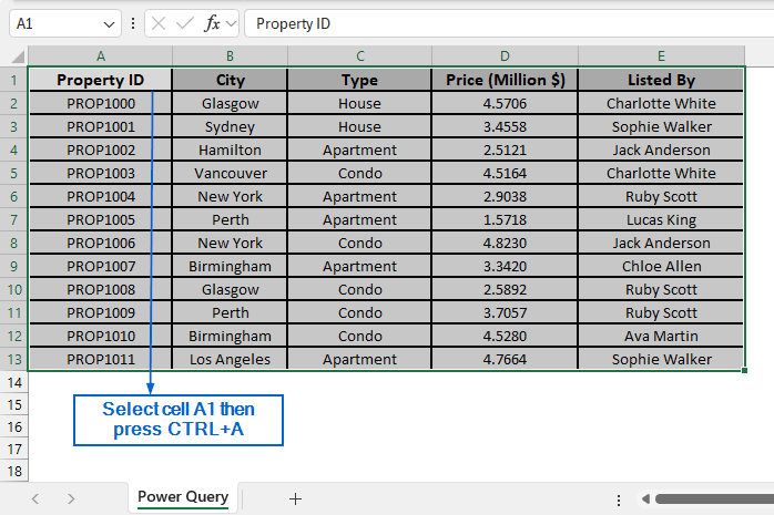
➤ Open the Power Query worksheet, click on cell A1 and press CTRL + A to select the entire dataset.
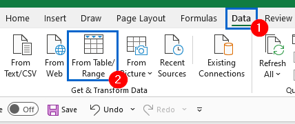
➤ Next, head to Data tab and click on the From Table/Range option.
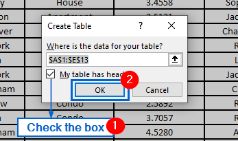
➤ In the Create Table dialogue box, check the My table has headers box and click on OK.
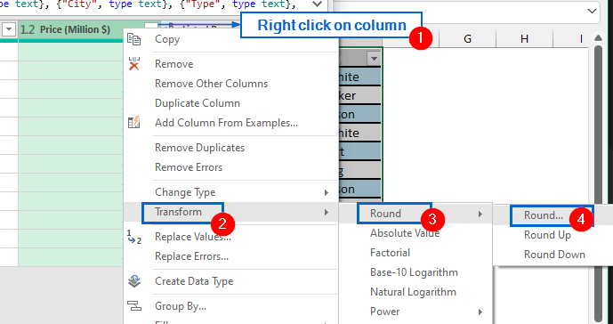
➤ In the Power Query Editor, navigate to the Price (Million $) column and right-click on it to bring out the context menu.
➤ From the context menu, head to Transform >> Round >> Round.
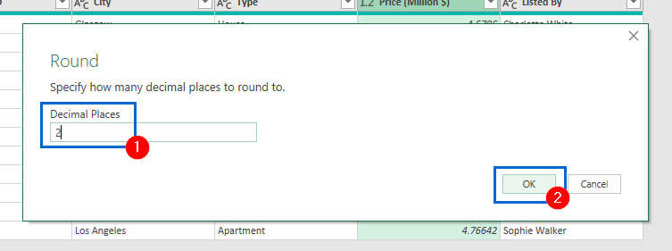
➤ Then type “2” in the Decimal Places box and click on OK to complete the operation.
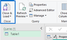
➤ Finally, click on the Close & Load button to import the dataset back to Excel.
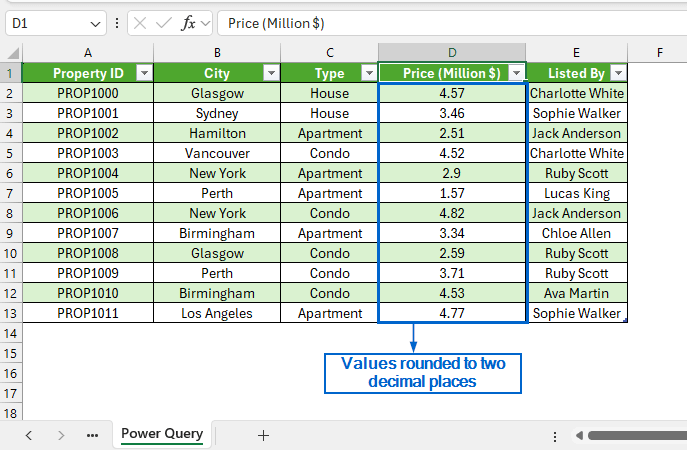
➤ The values in column D are now displayed rounded to two decimal places.
The same Round submenu holds two more options that formatting alone cannot reproduce. Round Up always moves a value away from zero, so 2.1 becomes 3, and Round Down always moves it towards zero, so 2.9 becomes 2. Both match Excel’s ROUNDUP and ROUNDDOWN functions, and neither asks for a decimal-places setting – they go straight to the next whole number. Use these when you need a value that is never lower, or never higher, than the original rather than simply the closest one. For the formula version, see how to round down to the nearest whole number.
Downloadable Resources
Get our practice workbook or necessary files that we have worked with to prepare this article.
Round Numbers Without Formula.xlsx
Frequently Asked Questions
Which Method is Best For Large Datasets?
When working with large datasets, Format Cells and Power Query methods are the most efficient. Unlike other methods, you do not need to manually select cells and apply formulas, helping you to save time and streamline workflows. Percentage columns behave differently from plain numbers, so if that is your data, see how to round percentages in Excel.
What is the Difference Between Rounding Numbers With and Without Formulas in Excel?
Rounding numbers using formulas such as ROUND, ROUNDUP, and ROUNDDOWN returns a genuinely rounded value in the cell holding the formula, and every later calculation that points at that cell uses the rounded number rather than the original. Your source column is left untouched. If Excel is rounding when you did not ask it to, here is how to stop Excel from rounding your decimals. Whereas rounding without formulas only changes the way the number is displayed (except for the Power Query method).
Concluding Words
Knowing how to round numbers in Excel without using formulas is essential for simplifying data presentation. In this article, we have discussed four important methods on how to round numbers in Excel, including Formatting Cells, Using Decrease Decimal Button, Using Number Format Dropdown and Power Query tool. Feel free to try out all these methods and select one that is best suited for your needs.