
If Excel is showing fewer decimals than you typed, the value itself is almost always intact – only the display has been shortened, and the full number is still sitting in the Formula Bar. There are three common reasons. The cell carries the Number, Currency or Accounting format, each of which shows two decimal places by default. The column is too narrow, so the General format shortens the display to fit. Or the entry ran past 15 significant digits, which is Excel’s storage limit, and the digits beyond that were replaced with zeros. Only the last of those three actually changes your data. Percentage columns behave differently again, because Excel stores a percentage as a decimal – if that is your data, see how to round percentages in Excel. While it provides a cleaner look, displaying the exact numbers can be essential for detailed scientific data, monetary transactions, or analytical calculations. With some minor changes, you can change this format and display decimals in their full form.
➤ Select the cells with decimals and click on the Home tab.
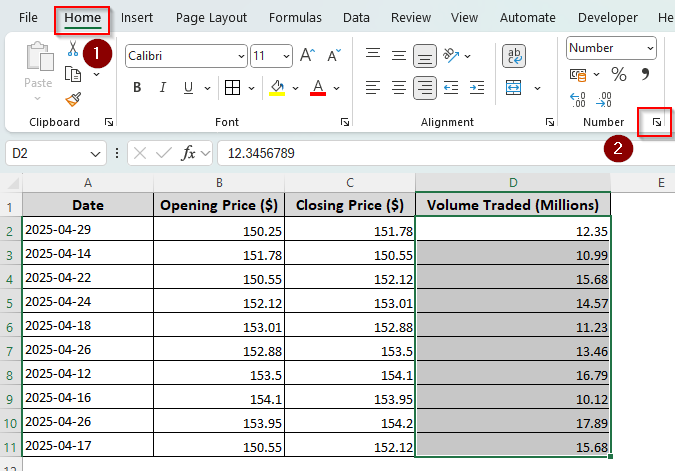
➤ From the top ribbon, locate the Number group and click the downward arrow (launch icon) to open the Format Cells options. Or, you can press CTRL + 1 .
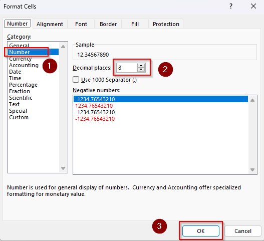
➤ As the Format Cells box appears, select Number. In the Decimal Places box, type how many decimal places to display in your dataset.
➤ Click Ok and Excel will display all the digits of your original numeric value without rounding up.
Other ways of preventing decimal roundup in Excel include fixing cell width, setting custom format, and using the TEXT function. In this article, we’ll cover each method step by step.
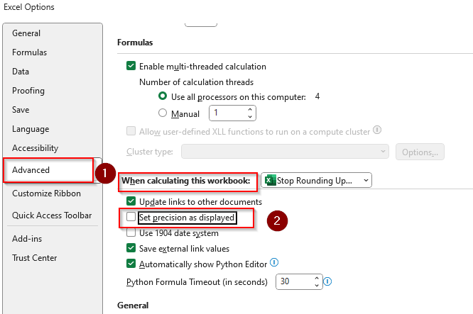
Remove the Set Precision As Displayed Setting to Avoid Decimal Roundup
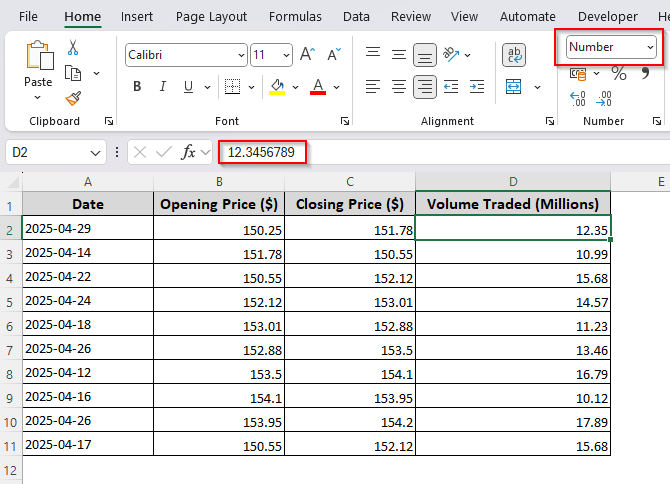
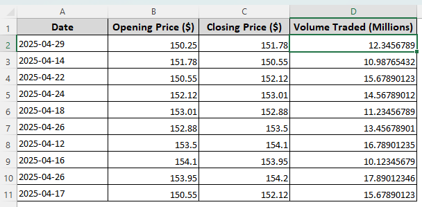
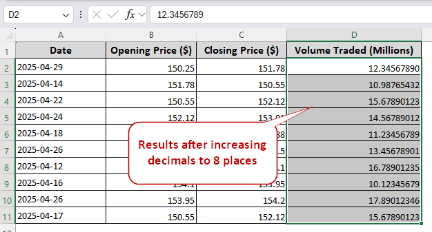
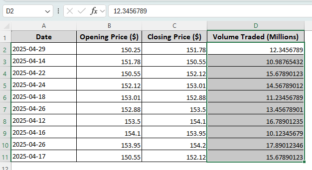
Our dataset contains 4 different columns of stock prices, volume, and related metrics. In Column D (Traded Volume), all our decimal numbers extend up to at least 8 decimal places.
As you can see, Excel has rounded up the decimals to two places even though they are formatted as Numbers. You can see the original value of the highlighted cell in the Formula box.
Before you load the decimal values in your worksheet, removing the Set Precision As Displayed setting can prevent data roundups. However, this won’t make any difference if you’ve already inserted your numeric values in the workbook.
Check this setting first, but do not expect it to be the culprit: it is switched off by default, so on most workbooks it was never the cause. It matters because of what it does when it is on – Excel permanently replaces each stored value with its displayed value, and those original digits cannot be recovered afterwards. Unchecking the box protects everything you enter from that point on; it cannot restore anything already overwritten. If a workbook has been running with it enabled, treat the affected figures as lost and re-import from the source. Here’s how to use it:
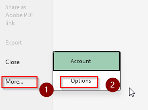
➤ Click on the File tab, choose More from the side column, and select Options.
➤ Go to Advanced and scroll down to locate the Set Precision As Displayed box in the When Calculating This Workbook group.
➤ Uncheck the box and click Ok. After that, you can load the decimals in your desired cells.
Fix Column Width to Display the Full Numeric Values
In some cases, not fixing the column width according to your data’s size can be the reason why Excel doesn’t display full numeric values.
Column width affects the two common cell formats differently, and it is worth knowing which you are looking at. A cell using the default General format shortens the number it displays until it fits the available width, which is what most people mean when they say Excel is rounding their numbers. A cell using a fixed format such as Number or Currency will not shorten the value, so it shows a row of hashtags (####) instead. Both are display-only, and clicking the cell shows the untouched value in the Formula Bar. The same formatting controls work in reverse when you do want fewer decimals – see how to round numbers without a formula. To fix this problem, follow the steps given below:
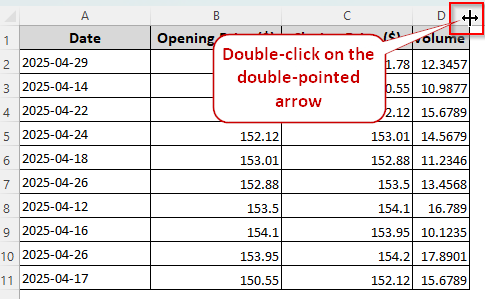
➤ Select the column with the decimal numbers and put your cursor on the right side of the column header.
➤ As the double-pointed + shaped arrow appears, double-click on it to readjust the size of the cells.
➤ When the cell extends, Excel displays the full numeric values as shown in the following image:
Using the Increase Decimal Feature to Adjust Decimals
Although this is the easiest method of adjusting the decimal places manually, it can be tiresome for large values. Here’s how to utilize the Increase Decimal feature effectively:
➤ Select the cells with the rounded decimal numbers and go to the Home tab.
➤ From the top ribbon, navigate to the Number group and click the Increase Decimal icon.
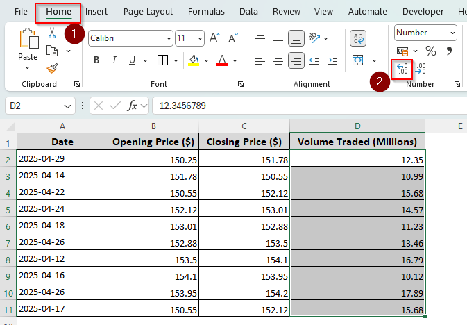
➤ Keep clicking on the icon until you get all the digits to display after the decimal point.
Format Cells and Specify Decimal Places
With the Format Cells option, you can convert your numeric values into numbers, currencies, scientific values, or accounting data. There’s also a custom formatting option.
No matter which format you choose, always specify the decimal places to prevent Excel from rounding up the decimals. Let’s get to the steps:
➤ Select all the cells with decimal numbers and click on the Launcher button in the Number group of the Home tab. You can also use the keyboard shortcut CTRL + 1 .
For Excel-Specified Formatting
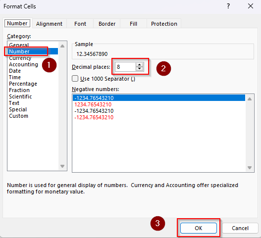
➤ In the Category section of the Format Cells box, choose Number, Scientific, Currency, or Accounting based on your sheet data. As we’re using decimal numbers, we selected the Number category.
➤ Go to the Decimal Places box and type a number or use the upward/downward arrow to specify how many digits you want to display after the decimal point. Click Ok.
For Custom Formatting
➤ Instead of selecting from the existing categories, you can click on Custom and enter 0.000000## in the Type box.
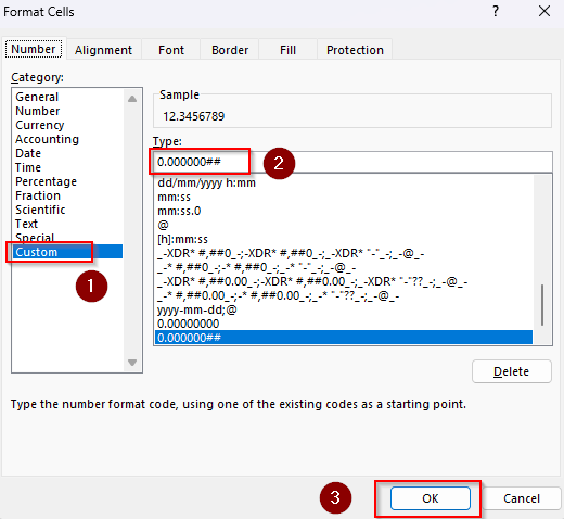
➤ This way, Excel will display 8 digits after the decimal point. The zeros represent the first 6 digits and the hashtags (#) represent the remaining 2 digits.
➤ Change the number of zeros and hashtags according to your dataset, keeping the code in the Type box. For example, to display up to 4 digits after the decimal point, enter 0.00## – two zeros that always show and two hashtags that appear only when there is a digit to fill them.
➤ Finally, press Ok.
In both cases, Excel displays the original numeric values up to your specified decimal places.
Apply the TEXT Function to Specify Decimal Places
With the TEXT function, we can create a formula that converts the decimal numbers into text and specifies the decimal places. Keep in mind that converting to text won’t allow you to perform accurate numeric calculations in Excel with this converted data. Here’s the process:
➤ Create a helper column and enter the following formula in the first cell adjacent to the first decimal number:
=TEXT (D2, “0.00000000”)
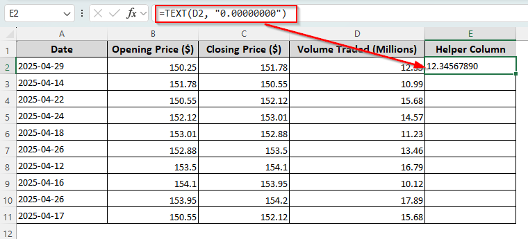
➤ Here, D2 is the cell reference containing the decimal number we’re converting. The number of zeros (0) after the decimal point represents how many digits we want to display after the decimal point. Change the values according to your dataset.
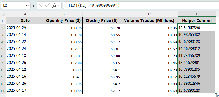
➤ Press Enter and use the tiny + sign (fill handle) on the bottom corner of your cell to drag and apply the formula to the remaining cells.
Display Large Decimal Numbers with Apostrophe
Excel stores numbers to 15 significant digits in every version on every platform. This is a published specification rather than a bug or a version quirk, so any digit past the fifteenth is replaced with a zero the moment you press Enter. If it is meaningful digits you need to control rather than raw length, see how to change significant figures. Excel rounds up the numbers or simply displays zeros (0) for any value you enter after the 15-digit mark. Using an apostrophe (‘) in the following way will fix this problem:
➤ For this method, we inserted a 15-digit decimal number in cell D2.
➤ As you can see, Excel doesn’t display the original value in the cell, but you can find it in the formula box when you click on the cell.
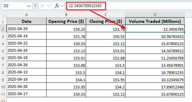
➤ To display the full numeric value in the cell, enter an apostrophe (‘) before the first number and press Enter.
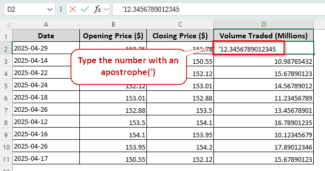
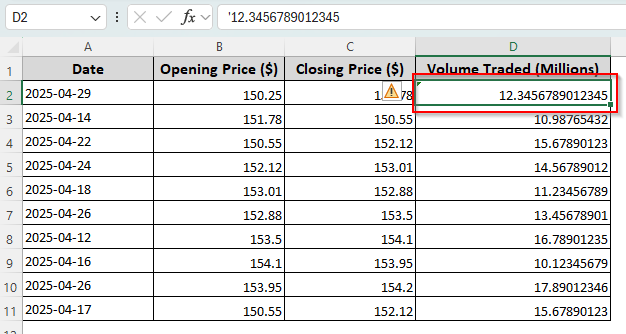
➤ Now, Excel displays the full decimal number without rounding up while also hiding the apostrophe.
Note:
Using an apostrophe also converts numerical data into a text string, so you’re unable to use it accurately for future calculations and formula applications.
Downloadable Resources
Get our practice workbook or necessary files that we have worked with to prepare this article.
Stop Excel from Rounding Up Decimals.xlsx
Frequently Asked Questions
How do I get rid of decimals in Excel without rounding?
Use a formula with the TRUNC function to remove decimals without rounding. In a helper column cell, type the following formula:
=TRUNC(D2, 0)
Replace D2 with the appropriate cell reference containing the decimal number. TRUNC always cuts towards zero, so if you want a genuine downward round instead, see how to round down to the nearest whole number. Instead of 0, you can use a whole number to specify how many decimal places you want to display.
How to remove scientific notation from large numbers in Excel?
Sometimes Excel rounds up large numbers and displays them as exponential E+ (example: 2.06578E+14). To avoid applying such scientific notations, select the cells and press CTRL + 1 to open the Format Cells window. Click on Number and type 0 in the Decimal Places box. Press Ok.
How do I stop Excel from turning decimals into dates?
To stop Excel from converting decimals to dates, you need to format your cells as numbers. Select the cells with decimals and click on the Home tab. Go to the Number group in the top ribbon and select Number in the cell format box, replacing the General or Date format. That prevents future entries from converting, but it does not undo one that already happened. Once Excel has turned an entry into a date it stores the date serial number, so switching the format to Number afterwards shows that serial rather than your original decimal. Clear the cell, apply the Number format, then type the value again.
Wrapping Up
To stop rounding up decimals in Excel, choose the correct method depending on how Excel rounds up data. In any case, formatting cells as numbers and specifying decimal places always work for any type of dataset.
However, it can be much simpler like changing the column width or adjusting decimals. Try each method keeping in mind the drawbacks we’ve mentioned.