
Calculating the elapsed time between two dates is a core task in Excel, whether you’re tracking project deadlines, analyzing employee work periods, or managing invoices. Without the right approach, it’s easy to get incorrect results, especially when switching between days, months, or hours.
In this article, we’ll show you multiple proven methods to calculate elapsed time between two dates. You’ll learn simple subtraction for total days, how to convert durations into hours, minutes, or seconds, and how to use the DATEDIF, NETWORKDAYS, and month-based formulas. Let’s begin.
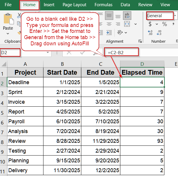
Steps to calculate elapsed time between two dates in Excel:
➤ Enter your start dates in column B and end dates in column C.
➤ Go to a blank cell like D2.
➤ To avoid the result appearing as a date instead of a number, select the cell, go to the Home tab >> Number group >> choose General.
➤ Type the formula: =C2-B2
➤ Press Enter.
➤ Drag the fill handle down to apply to other rows.
Subtract Dates Directly to Calculate Days Between Two Dates
Subtracting one date from another is the simplest way to calculate elapsed days in Excel – the same logic applies within a single day when you calculate the difference between two times. Excel stores dates as serial numbers, so subtracting the start date from the end date instantly gives the number of days between them. This is ideal when you need a fast calculation without extra functions or formatting.
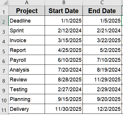
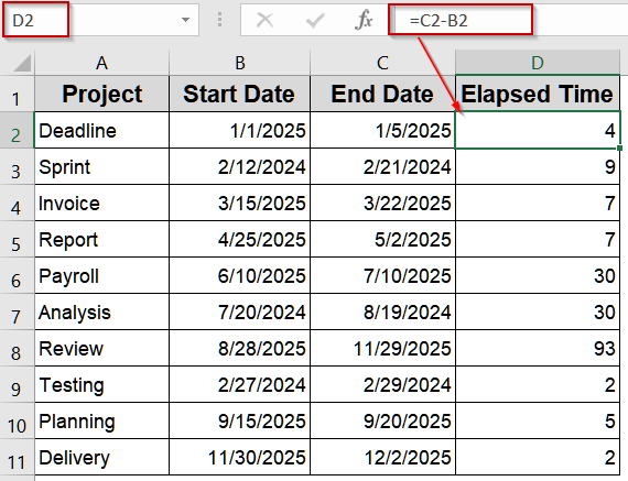
We’ll use the following sample dataset:
Steps:
➤ Enter your start dates in column B and end dates in column C.
➤ Go to a blank cell like D2.
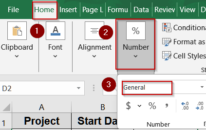
➤ To avoid the result appearing as a date instead of a number, select the cell, go to the Home tab >> Number group >> choose General.
➤ Type the formula:
=C2-B2
➤ Press Enter.
➤ Drag the fill handle down to apply to other rows.
Multiply Subtracted Days to Get Total Hours, Minutes, or Seconds
Once you have the difference in days, multiplying by conversion factors can convert it to hours, minutes, or seconds. This is essential for performance metrics or process timing where finer units matter.
These factors come into their own when your cells hold a date and a time together, such as 1/1/2025 9:00 and 1/3/2025 14:30, because the subtraction then returns 2.229 days rather than a whole number. Multiplying by 24 turns that into 53.5 elapsed hours. If you would rather read it as days, hours and minutes, format the result cell as Custom with the code d" days "h:mm, which displays 2 days 5:30 for any span shorter than 32 days – and use [h]:mm instead (53:30 here) when you want the whole span expressed in hours without the days split out. That combined date-and-time case is covered in full in how to subtract date and time in Excel.
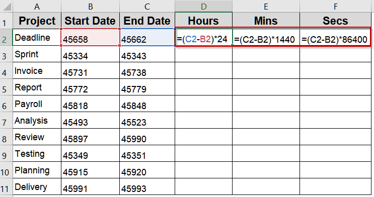
Steps:
➤ Enter your start dates in column B and end dates in column C.
➤ Go to a blank cell like D2.
➤ To calculate hours, type this formula:
=(C2-B2)*24
➤ For minutes, use this formula in E2 cell:
=(C2-B2)*1440
➤ For seconds, use this formula in F2 cell:
=(C2-B2)*86400
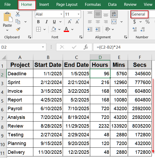
➤ Format the result cell as General from the Home tab.
➤ Press Enter and drag the fill handle down for all rows.
Use DATEDIF Function for Full Days, Months, or Years
The DATEDIF function provides elapsed time directly in specific units such as days, months, or years. This method is particularly useful for calculating ages, project phases, or HR data where full units are needed.
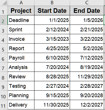
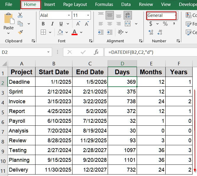
It is an unusual function: Microsoft kept it only to support older Lotus 1-2-3 workbooks, so it never appears in Formula AutoComplete and you will not find it in the function list. Type it in full and it works in every version. For a plain day count, subtracting one date from the other as in Method 1 is Microsoft’s own recommendation. We’ll use this modified dataset for demonstration:
Steps:
➤ Place start dates in column B and end dates in column C.
➤ Click a blank cell like D2.
➤ To calculate days, type this formula:
=DATEDIF(B2,C2,"d")
➤ For months, use this formula in E2 cell:
=DATEDIF(B2,C2,"m")
➤ For years, use this formula in F2 cell:
=DATEDIF(B2,C2,"y")

➤ Press Enter and copy down.
➤ Format the result cell as General from the Home tab.
Combine DATEDIF Units to Display Years, Months, and Days Together
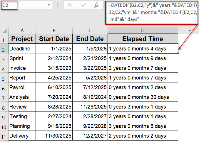
You can merge multiple DATEDIF function calculations to show elapsed time in a single readable string like “2 years 5 months 3 days”. This is especially handy for service anniversaries or detailed timeline reports.
One caution on the last component. Microsoft does not recommend the "md" unit, because it ignores months and years entirely and can return a negative day count when the end date falls earlier in its month than the start date does – 31 January to 1 March is the classic case. For anniversaries and service dates the formula below is reliable, but spot-check any row where the start date is near the end of a month.
Steps:
➤ Enter start dates in B2 and end dates in C2.
➤ Select a blank cell such as D2.
➤ Format the result cell as General from the Home tab under the Number group.
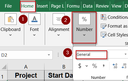
➤ Type this formula:
=DATEDIF(B2,C2,"y")&" years "&DATEDIF(B2,C2,"ym")&" months "&DATEDIF(B2,C2,"md")&" days"
➤ Press Enter.
➤ Drag the fill handle to fill down.
Calculate Date Difference in Weeks Using DATEDIF and ROUNDDOWN Functions
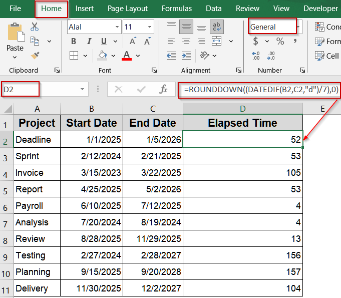
When you need the elapsed time in weeks, dividing the day difference by seven and rounding down gives whole weeks. This is useful for tracking weekly sprints or schedules.
Steps:
➤ Enter start dates in B2 and end dates in C2.
➤ Click an empty cell like D2.
➤ Type this formula:
=ROUNDDOWN((DATEDIF(B2,C2,"d")/7),0)
➤ Press Enter.
➤ Format the cell as General and drag down.
Compute Months Between Two Dates Using YEAR and MONTH Functions
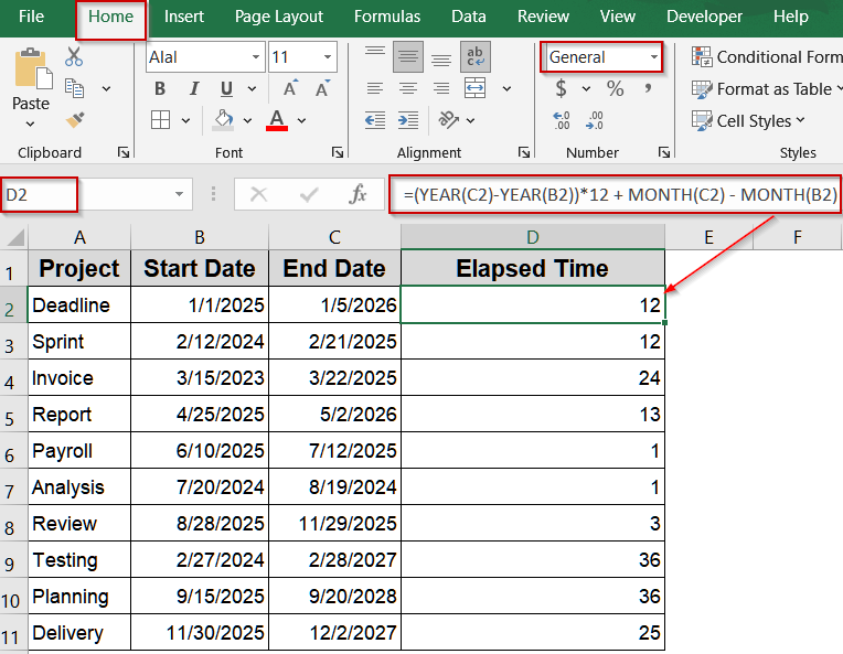
This counts how many calendar month boundaries the range crosses, which is a different question from the one Method 3 answers – and the two will disagree. DATEDIF with "m" counts complete months, so 15 June 2024 to 14 June 2025 returns 11 because the final month has not finished. This formula counts boundaries, so the same pair returns 12. Use DATEDIF when a month only counts once it is fully served, such as tenure or age, and use this one for billing periods where crossing into a new calendar month is what triggers the charge.
Steps:
➤ Put start dates in B2 and end dates in C2.
➤ Select a blank cell like D2.
➤ Type this formula:
=(YEAR(C2)-YEAR(B2))*12 + MONTH(C2) - MONTH(B2)
➤ Press Enter and drag the fill handle down.
➤ Format the cell as General for correct display.
Use NETWORKDAYS to Calculate Duration in Working Days
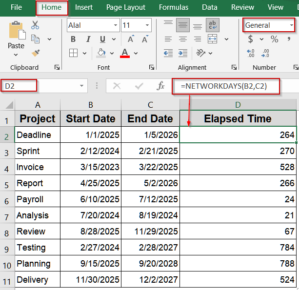
If you only need to count Monday to Friday workdays across a date range, the NETWORKDAYS function is the correct choice. It’s frequently used in project planning or payroll to exclude weekends automatically.
Note that it counts both the start and the end date, not the gap between them. A Monday-to-Friday range returns 5, and the same working day entered twice returns 1 rather than 0. If you want the elapsed days excluding the start date, subtract one. It also ignores any time values in the cells, and if your weekend is not Saturday and Sunday, use NETWORKDAYS.INTL instead, which lets you specify which days count as the weekend. To turn workdays into billable hours, see how to calculate total hours in Excel.
Steps:
➤ Enter your start dates in B2 and end dates in C2.
➤ In a blank cell like D2, type this formula:
=NETWORKDAYS(B2,C2)
➤ Press Enter.
➤ Drag the fill handle to copy for all rows.
➤ Format as General for a clean numeric result.
Downloadable Resources
Get our practice workbook or necessary files that we have worked with to prepare this article.
Calculate Elapsed Time Between Two Dates in Excel.xlsx
Frequently Asked Questions
Is Excel’s date arithmetic accurate with leap years?
Yes. Excel date serial numbers automatically account for leap years. Subtraction, DATEDIF, and NETWORKDAYS functions include February 29 when applicable, so calculations spanning leap years remain accurate without requiring manual adjustments or additional formulas.
How do I calculate elapsed time in days between two dates in Excel?
Use a simple subtraction formula such as =End_Date-Start_Date (e.g., =C2-B2). If the result displays as a date, format the cell as General or Number to view the total elapsed days accurately.
What is the DATEDIF function used for when calculating elapsed time?
The DATEDIF function directly calculates differences in chosen units. For example, use =DATEDIF(A2,B2,"d") for days, "m" for months, or "y" for years. It’s ideal for precise elapsed calculations spanning multiple months or years effectively.
How can I calculate elapsed time in weeks between two dates?
Use the formula =ROUNDDOWN(DATEDIF(A2,B2,"d")/7,0) to convert total days into full weeks. This divides the day difference by seven, then rounds down. It’s perfect for schedules, timelines, or weekly reporting in Excel.
What formula should I use for business or working days only?
Use =NETWORKDAYS(Start_Date,End_Date) to count weekdays, excluding Saturdays and Sundays. Remember it counts both the start and end dates. To exclude specific holidays as well, include a holiday range such as =NETWORKDAYS(Start_Date,End_Date,Holiday_Range).
Wrapping Up
In this tutorial, we explored several reliable ways to calculate elapsed time between two dates in Excel, including direct subtraction for days, multiplying by 24, 1440, or 86400 for hours, minutes, or seconds, and using DATEDIF function for years, months, and days. We also covered NETWORKDAYS function for business days and a combined DATEDIF formula for detailed differences. Feel free to download the practice file and share your feedback.