Are you looking for a simple solution to master your schedules, calculate work hours, and manage time effortlessly? Google Sheets time formulas will help you add, subtract, and format time values just like clockwork in a well-oiled machine. Functions like TIME, NOW, and TEXT will simplify your time management, perfectly tracking hours, schedules, and event durations. Without wasting time, let’s dive in and unpack the nuts and bolts of Google Sheets time formulas.
Determining Time Difference in Google Sheets
While working on a project, you may need to add or subtract time to account for the time difference. This may be hectic if you are not familiar with all the techniques. Here, we have discussed all types of methods you will find for calculating time duration. Without moving here and there, let’s dig into it.
Subtract Time
In order to get the difference between two times, you just need to subtract the time values from both cells.
➤ Select a cell and type the formula below.
=D2-C2
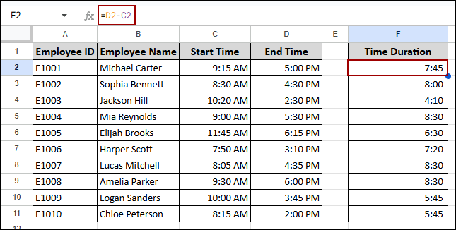
This way, we will find the time difference for the starting and ending times for the employees.
Using TEXT Function
The TEXT function is used to format numbers, dates, and times into a specific text format. In this part, we will calculate the time difference and then format it into different formats for hours, minutes, and seconds.
First, let’s find the time difference and format for the hour value.
➤ Select a cell and write the formula below.
=TEXT($D2-$C2,"h")
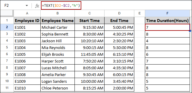
As you can see, you will be displayed only the hour differences for the start and end times.
Now we will determine the difference between the two times, but this time we will format it as hh: mm.
➤ For this, choose a cell and put the formula below.
=TEXT($D2-$C2,"hh:mm")
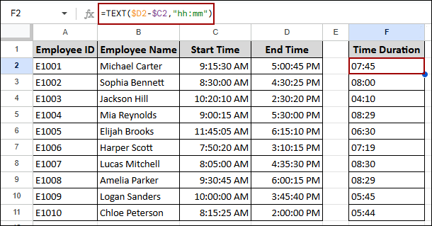
Thus, we will get the time difference shown as hours and minutes.
Now, we will format the time value and display hours, minutes, and seconds.
➤ Just select a cell and type the formula, and click ENTER.
=TEXT($D2-$C2,"hh:mm:ss")
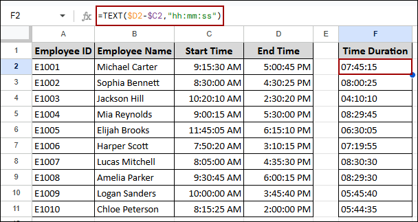
Finally, the time differences will be shown with hours, minutes, and seconds.
Calculating Time Difference in Hours, Minutes, and Seconds
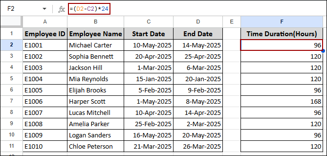
In some places, you might need to calculate the time differences into hours, minutes, and seconds. Well, you don’t need to calculate first and then convert the value to your desired output. With just a single formula, you can make it happen instantly.
➤ Click a cell and write down the formula below.
=(D2-C2)*24
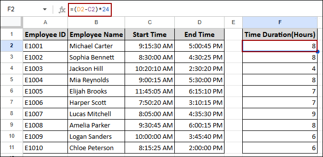
This way, multiplying the time differences by 24, you will get the hour values only.
Note:
Here, the hours will be rounded, ignoring the minutes.
Similarly, you can get the minute value only by multiplying the time by 1440.
➤ Choose a cell and put the formula below.
=(D2-C2)*1440
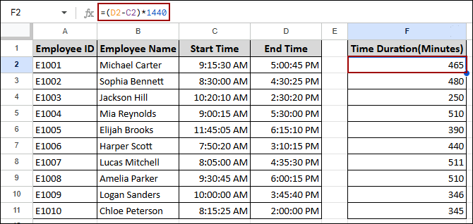
As you can see, we have successfully extracted the time differences into minutes.
In order to get seconds, you just need to multiply by 86400.
➤ Click a cell and apply the formula below.
=(D2-C2)*86400
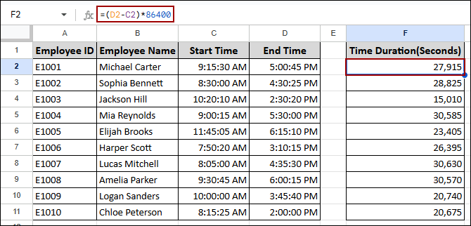
Finally, the selected cell will display the time duration in seconds.
Applying HOUR Function
While working, you might need to extract only the hour from two given times. Google Sheets’ HOUR function will provide you with the exact solution for this.
First, let’s calculate the time duration between two times and extract only the hours. To do so,
➤ Choose a cell and put the formula below.
=HOUR(D2-C2)
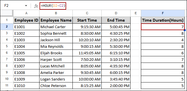
Thus, we have successfully taken out the hours in a new column.
Note:
The HOUR function first calculates the total time and then extracts only the hour.
Time Difference Between Two Dates
You can monitor durations, deadlines, or age in Google Sheets by calculating the time difference between two dates. Just subtracting one date from another can achieve this. Depending on the requirement, the output can be prepared to display the difference in days, hours, or other units. In this part, we will calculate the time difference in hours.
➤ Simply, choose a cell and write down the formula.
=(D2-C2)*24
Thus, you will get the time duration in hours between the two dates. In order to get the time differences in minutes and seconds, you can multiply the difference by 1440 and 86400.
Adding or Subtracting Time Using TIME Function
The TIME function in Google Sheets is used to pull out a specific time value using hours, minutes, and seconds. As it takes hours, minutes, and seconds as its components, you can add or subtract your desired time with this function.
Hours
In this section, we will add hours using the TIME function.
➤ Choose a cell and put the formula below.
=C2+TIME(8,0,0)
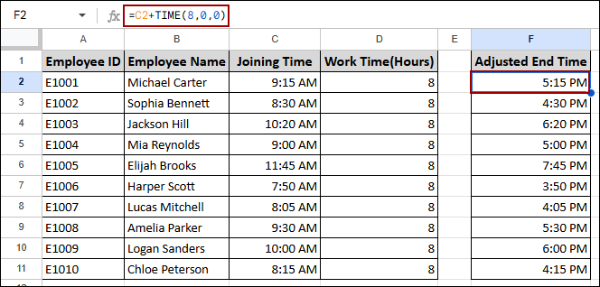
As you can see, we have successfully added 8 hours with their joining time.
Minutes
Similarly, you can add minutes to a time in Google Sheets. Just provide the value in the minute component section, and the minutes will be added.
➤ Select a cell and write down the formula below.
=B2+TIME(0,45,0)
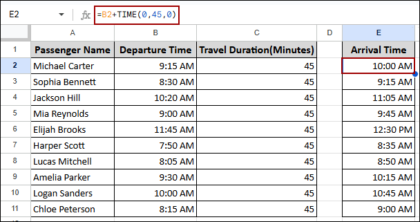
Finally, the minutes will be added with the departure time.
Seconds
This time, we will add seconds using the TEXT function.
➤ Choose a cell and write down the formula below.
=B2+TIME(0,0,220)
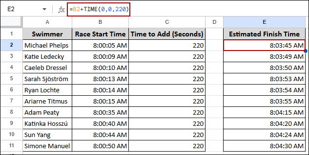
As a result, we will get the output adding 220 seconds to the start time.
Calculating Total Time Using SUM Function
In some situations, you might need to compute the total time. The SUM function can calculate the total time without any hesitation. Here, we will use the SUM function to calculate the total time spent in Google Sheets.
➤ Click a cell and write the following formula.
=SUM(D2:D11)
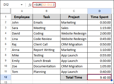
Thus, you will get the total time.
Summing Hours over 24 Using TIME Function
The TIME function is utilized to create a specific time value. But when the hour value exceeds 24, the TIME function resets it back to 0 and displays the relevant time. In this situation, you need to calculate the days first and then use the TIME function to get the time.
➤ First, choose a cell and write the following formula.
=INT(C3/24)
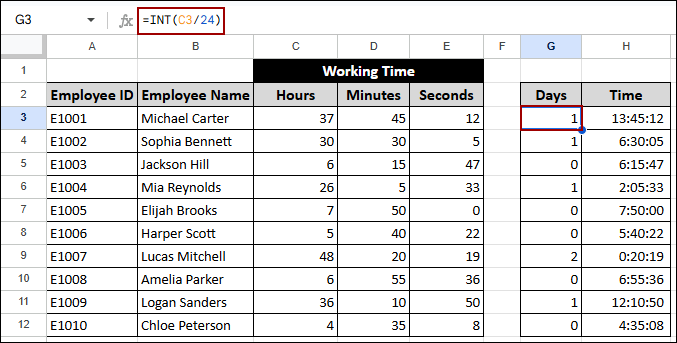
➤ Now, use the following formula in another cell to get the time.
=TIME(C3, D3, E3)
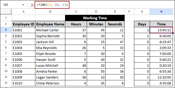
Thus, you will get the total days spent for the hours exceeding 24 and the correct time applying the TIME function.
Extracting Date and Time Using ROUNDDOWN Function
Sometimes you will get to see the date and time in the same cell. Thus, if you want to get the date and time in two different cells, you can use the ROUNDDOWN function. The ROUNDDOWN function with 0 decimal places removes the time portion from a date-time value.
➤ Select a cell and put the following formula.
=ROUNDDOWN(C2, 0)
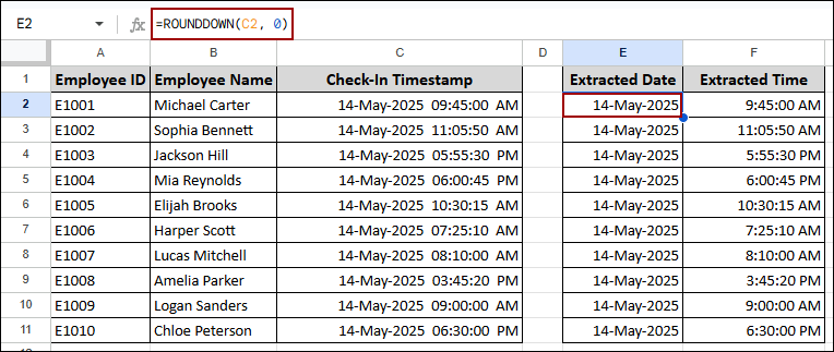
➤ Now, put the formula below to get the time differences in another column.
=C2-E2
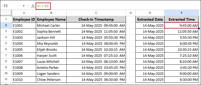
Thus, you will get the date and time extracted from a date-time value.
Apply Timezone with Google Sheets Apps Script
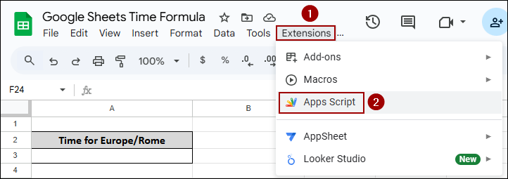
Timezone management is crucial when collaborating across regions and arranging events. To work with different time zones, you can use Apps Script to adjust time according to multiple regions. Here, we will extract the time for Europe with Apps Script. If you want, you can add any timezone inside the formula to get your desired date and time.
➤ Start by clicking Extensions > Apps Script from the menu bar.
➤ Then, put the code below and click Save.
function nowtimezone(timeZone) {
return Utilities.formatDate(new Date(),
timeZone, "yyyy-MM-dd HH:mm:ss");}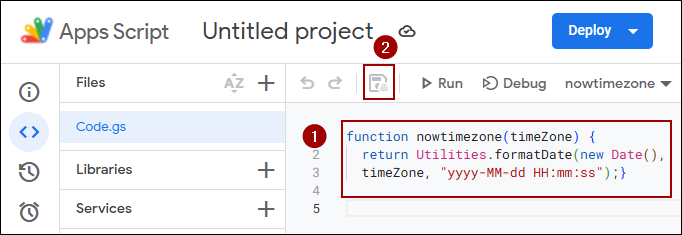
➤ After that, coming back to the spreadsheet, put the formula in a cell.
=nowtimezone("Europe/Rome")
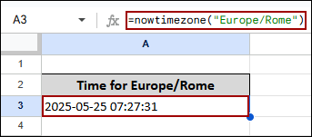
Thus, you will get the date and time for the Europe/Rome timezone.
Formatting Time in Google Sheets
Sometimes, you might not get the appropriate format displayed for the date and time you wished for. This happens when the cell format is not chosen properly. For this, you need to change the format according to your demand. You can do it easily as Google Sheets has multiple formats like hh: mm, hh:mm: ss, hh: mm AM/PM. You can also use the Custom Format option to get the specific format for your audience.
➤ From the Menu bar, click Format > Number.
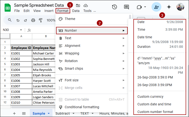
Now, choose your desired format that you want to represent for the chosen cells.
Frequently Asked Questions
Why is my time calculation showing ######?
This happens when the output is negative, which Google Sheets can’t display as time. You can check for reversed start and end times, or use ABS() for absolute values, or an IF() formula to avoid negative values.
Can I use conditional formatting based on time values?
Yes, you can use conditional formatting based on time values. For this, inside the formatting rule option, use a formula like this =A1<TIME(9,0,0) to highlight times earlier than 9:00 AM. Similarly, you can adjust the values for minutes and seconds. Please make sure the cell is formatted as Time.
Can I calculate the average of time values?
Of course, you can calculate the average of time values using the AVERAGE function. To get the appropriate format, pre-format the cells as Time before entering the values.
Conclusion
Google Sheets has all the built-in time formulas to track, calculate, and format time values according to your needs. In this article, I have covered solutions for all the scenarios where you might face difficulties using time formulas. If you find any problems regarding time formulas, don’t forget to share in the comment section below. Thanks!