With Google Sheets, autofill allows you to enter data without having to type it all by hand. When working with numbers, dates, or the days of the week, autofill can be used to extend cells. It can also be used to duplicate formulas between cells. To use autofill, you must first enter data in a cell, then select the cell and move the fill handle—a tiny blue square—in the direction you want. Google Sheets will automatically identify the pattern and execute it for you. This article will show us how to utilize Autofill effectively and provide some time-saving data handling advice.
What Is Autofill Feature in Google Sheets?
Applying a pattern or current data, Google Sheets automatically fills in cells with data. This method saves you time and effort by copying formulas or continuing sequences. Cells can be filled with Autofill:
- Number sequences, such as 1, 2, 3, etc.
- Weekdays, such as Monday, Tuesday.
- Months, such as January, February, etc.
- Dates. For example, 01/01/2025, 02/01/2025, etc.
- Copying numbers or text between cells
- Extending basic formulas
- Repeating a single value
- Rapidly filling rows or columns
- Making dropdown lists (with data validation)
- Smart Fill (AI-supported pattern suggestions)
Autofill Based on Another Field in Google Sheets
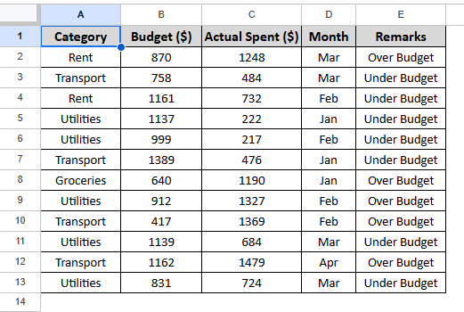
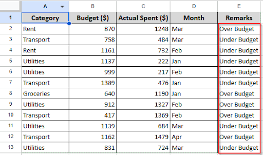
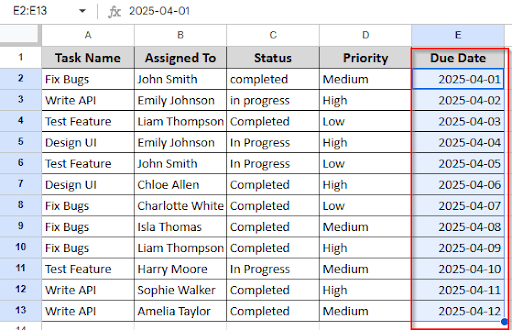
In Google Sheets, you can autofill cells based on a particular column or a range of cells very quickly. You can use formulas like IF or VLOOKUP to check conditions and return values properly. You can apply the fill handle to copy formulas or values to autofill a cell based on the value of another cell. Let’s look at the dataset below, where every entry is currently in its default format.
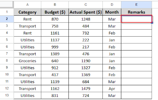
Here, if we want to autofill based on another field, what we have to do is:
➤ Start with the “IF” formula in the first row. Click on the first empty cell under the Remarks column (let’s say cell E2)
➤ Enter this formula in cell E2:
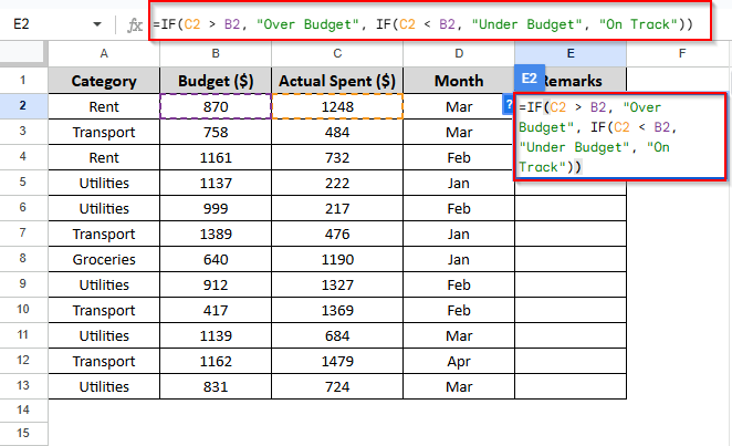
This formula will return:
- If Actual Spent > Budget, then return “Over Budget”
- If Actual Spent < Budget, then return “Under Budget”
- If they are equal, return “On Track”
Here, C2>B2; that means the actual spent is greater than the budget, for which it returns over budget in the remarks column.
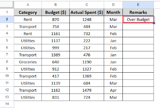
➤ Use the Fill Handle to Autofill
➤ After entering the formula in E2, click on the cell.
➤ Move your mouse to the bottom-right corner of the cell until you see a small blue square (the fill handle).
➤ Click and drag the handle down to apply the same formula to the rest of the rows.
Google Sheets will automatically adjust the row numbers (C3, B3, C4, B4, etc.) and apply the logic for each row.
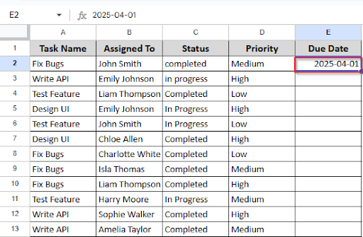
Autofill Dates in Google Sheets
In Google Sheets, auto-filling dates allows you to avoid manually typing each date by enabling the sheet to maintain a date pattern automatically. It lets you rapidly construct a complete list of dates and saves time.
➤ In the Due Date column (Column E), type your starting date.
Example: 2025-04-01 in cell E2.
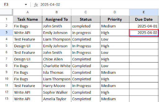
➤ In the next cell (E3), type the next date in the pattern. Example: 2025-04-02
➤ Now, select both cells (E2 and E3).
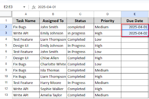
➤ Move your cursor to the bottom-right corner of the selection until you see the blue square (fill handle).
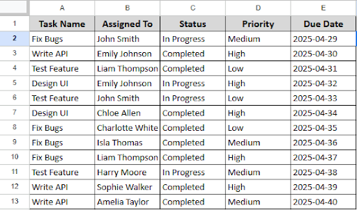
➤ Click and drag the fill handle down the column — Google Sheets will continue the date pattern for the rest of the tasks.
Autofill Dates When the Cell Is Updated
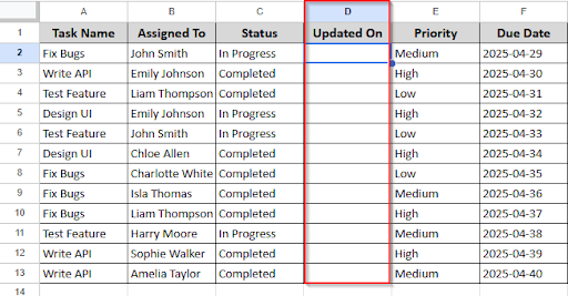
You might expect Google Sheets to automatically update the current date whenever you make changes to a single cell. Monitoring updates, job completion, or dataset revisions have become easier with this functionality. It’s not an integrated feature, but Google Apps Script makes it easy to use. Look at the dataset below, where all of the entries are in their default format at the moment.
Suppose you would like to have the current date automatically entered in a new column each time a cell in the Status column (Column C) is modified. What you have to do is:
➤ Insert a new column after Status (Column C) and name it: Updated On. It will become Column D (and the existing columns will shift right). For that, you have to right-click on Column C . Then a pop-up will come, and you have to click the “insert one-column-right” option. A new column will be created in Column D.
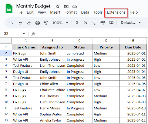
➤ Click Extensions > Apps Script.
➤ Delete anything already in the editor.
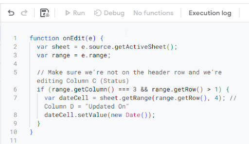
function onEdit(e) {
  var sheet = e.source.getActiveSheet();
  var range = e.range;

			Note: Make sure we're not on the header row and we're editing Column C (Status)

  if (range.getColumn() === 3 && range.getRow() > 1) {
    var dateCell = sheet.getRange(range.getRow(), 4); // Column D = "Updated On"
    dateCell.setValue(new Date());
  }
}
➤ Paste the full script on Apps Script.
➤ Click the Save icon and give your project a name.
➤ Close the editor.
To get the result:
➤ Go back to your sheet.
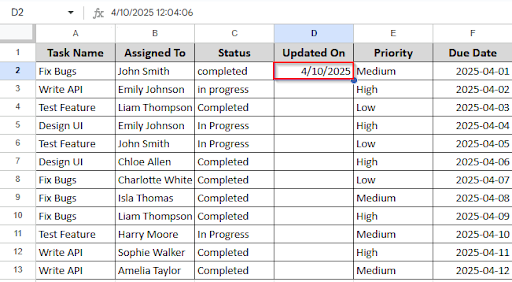
➤ In any cell in Column C (Status) — try changing “In Progress” to “Completed” or anything else.
➤ You should now see the current date appear in Column D (Updated On).
Adding a Serial Number in Google Sheets
Adding serial numbers to your Google Sheets data makes it easier to keep everything organized. Working with lists like student names, attendance, or inventory makes it easier to keep track of entries, count rows, and refer to information.
Although there isn’t a “serial number” option in Google Sheets, but you can do it with a few simple steps. There is a technique that works for you; you can do it manually by typing 1 and then dragging it, otherwise use a formula. Let’s say you want to generate serial numbers automatically using a formula. Here’s what you have to do:
➤ Insert a new column where you want the serial numbers.
➤ In the first cell under the header (e.g., A2), type
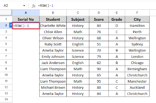
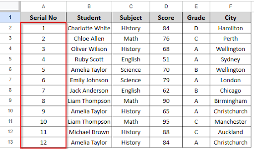
➤ Press Enter, then drag the fill handle down to apply the formula.
Autofill in Google Sheets without Dragging Cells
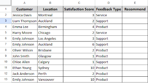
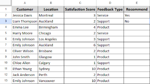
It can take a lot of time to manually slide the fill handle in Google Sheets, especially when dealing with big datasets. Fortunately, auto filling cells with built-in functionalities is simpler and doesn’t require dragging at all. Quick keyboard shortcuts and the ARRAYFORMULA function make it simple to autofill formulas rather than dragging them down a column with the mouse. Let’s look at the dataset below, where every entry is currently in its default format.
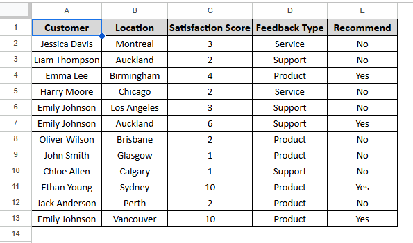
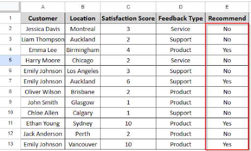
Suppose you have a table with customer details, including a Satisfaction Score in Column C. Now you want to autofill the “Recommend” column (Column E) with “Yes” if the score is 4 or higher, and “No” otherwise.
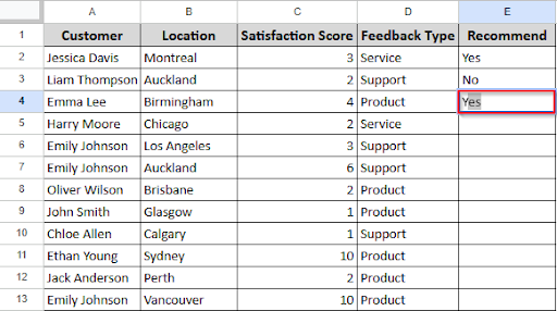
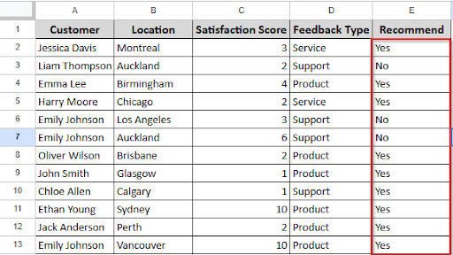
➤ Instead of dragging it down manually, you can use this formula in cell E2:
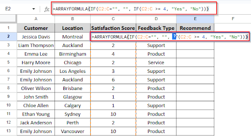
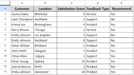
➤ No dragging is required once you enter this in E2, as the entire column fills automatically based on the values in Column C.
Smart Fill in Google Sheets
Smart Fill, a brilliant feature in Google Sheets, can magically fill in the blanks by automatically identifying patterns in your data. It functions similarly to autocomplete, but specifically for cells. Google Sheets can recognize a pattern you start entering in a column and automatically fill in the rest of the information. Particularly when working with organized or repetitive data, this minimizes errors and saves time. Let’s consider this dataset to understand how smart fill works.
➤ In the Recommend column, manually enter a few values based on the Satisfaction Score and Feedback Type.
➤ Following a few entries, Google Sheets will use the pattern you’ve created to automatically recommend values for the remaining cells in the Recommend column. A pop-up window with a recommendation will show up.
➤ To apply Smart Fill, press Ctrl + Enter if the recommendation appears to be accurate. The remaining column will be automatically filled in.
Autofill a Formula in Google Sheets
Probably you’ve already noticed how tiresome it can be to input the same formula repeatedly in Google Sheets. Fortunately, autofill is a quick and easy approach to save time. With this useful tool, you can easily apply a formula to a whole column without having to do it by hand for every row. Autofill takes care of all the repetitive calculations, whether you’re working on scores, totals, or anything else. To help you understand it in a practical example, we’ll demonstrate its application with a dataset of customer reviews in this example.
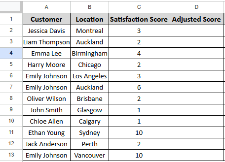
Let’s consider this dataset where everything is in its default format.
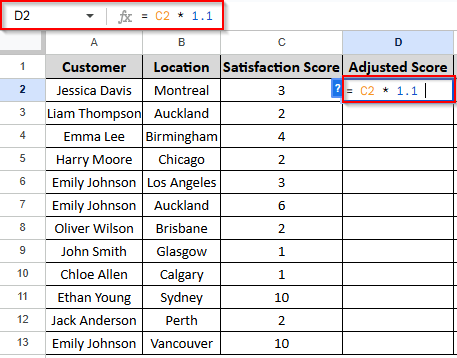
➤ Now, we want to create a new column that shows the Adjusted Score, which is the Satisfaction Score increased by 10%.
➤ In a new column (e.g., Adjusted Score), click on the first empty cell next to the first Satisfaction Score.
➤ Type the formula in cell D2:
➤ Press Enter to apply the formula.
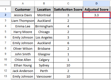
➤ Select the cell with the formula again. Hover over the bottom-right corner until you see a small + sign (the fill handle).
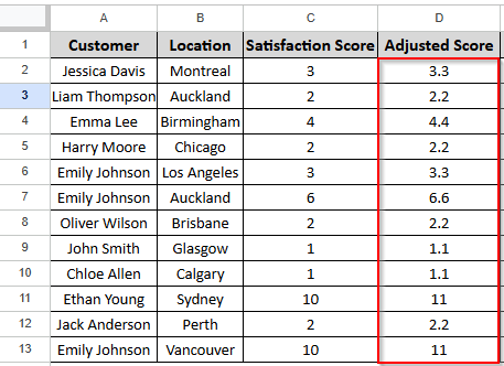
➤ Click and drag the fill handle down or double-click the fill handle through the rest of the column. The formula will automatically adjust for each row.
Frequently Asked Questions
How to turn on Autofill in Google Sheets?
Autofill is typically activated by default in Google Sheets. Google Sheets will automatically identify and recommend the remaining information when you start typing. After selecting the cell containing your data or formula, drag the fill handle to initiate autofill. By Double-clicking, you can also fill automatically.
How Do I Fill a Column Automatically in Google Sheets?
Enter your formula or value in the first cell, then double-click the fill handle to fill the column automatically. This will use the nearby data to automatically fill up the column.
Is there any keyboard shortcut for Autofill in Google Sheets?
There isn’t a keyboard shortcut; by using the fill handle, you can autofill quickly. The process is: You have to enter your value or formula in a cell.
- Press Ctrl + Enter for Windows, Cmd + Enter for Mac
- Also, by double-clicking the fill handle, you can autofill down.
Concluding Words
The Autofill feature allows you to quickly duplicate your work without having to do it by hand. It helps you stay organized and saves time when you fill in patterns or duplicate formulas. It eliminates the repetitive processes of using Google Sheets and enables you to quickly complete rows or columns.