To perform various calculations and manipulations on dates and times, Google Sheets provides a wide range of date functions and formulas. You can add or subtract days to count days between two dates, or extract specific details like the weekday name, month name, or week number from a given date. You can also find the last or first day of a month, calculate months between dates, and so on with different date formulas.We will try to discuss them briefly throughout the whole article.
Getting Weekday Name from Date in Google Sheets
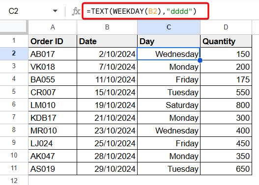
In our day to day life, we often feel the necessity of converting a date to a weekday name. In Google Sheets, we can do it easily with a simple formula combined with the WEEKDAY and TEXT functions.
To have weekday name from date in Google Sheets, go through the following procedures:
➤ Select a cell (i.e. C2) first.
➤ Write the following formula:
=TEXT(WEEKDAY(B2),"dddd")
Where, the WEEKDAY function returns a number representing the day of the week for a given date. The TEXT function converts a number into a text format and “dddd” is a date format code that represents the full weekday name.
➤ Press Enter to have the weekday name.
➤ Then, use Fill Handle to AutoFill the remaining cells.
Convert Week Number to Date in Google Sheets
In Google Sheets, you can convert a week number to date quite easily. You need to use the DATE and WEEKDAY functions for this purpose.
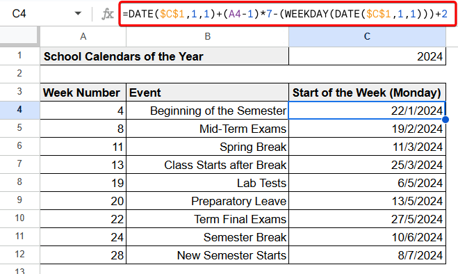
Here, we have a school calendar for the year 2024. We will convert the week number of a certain event to an actual date. We will consider Monday as the first day of the week.
To convert the week number to date in Google Sheets, apply the following formula:
=DATE($C$1,1,1)+(A4-1)*7-(WEEKDAY(DATE($C$1,1,1)))+2
Where, $C$1 signifies the year value (i.e. 2024) and A4 signifies the week number.
Current Date Formula in Google Sheets
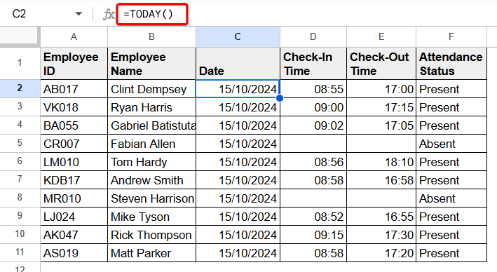
In Google Sheets, you can easily get the current date. The TODAY function is fully dedicated for this purpose.
To get the current date in Google Sheets, apply the following formula:
=TODAY()
Count Days from Date to Today in Google Sheets
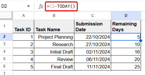
TODAY function returns the date of that particular day. To count days from date to today, you can subtract the date from today’s date to count the date.
Just write the following formula and press Enter to count days:
=C2-TODAY()
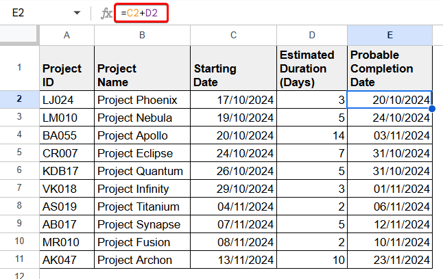
Add Days to Date in Google Sheets
Adding days to date is a very easy and simple task in Google Sheets. With basic additional formula, you can add days to date.
To add days in date, just use the following formula:
=C2+D2
Where, C2 defines date and D2 defines the days to be added.
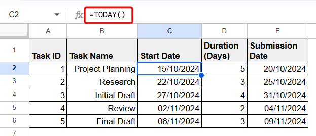
Add Dates in Google Sheets Automatically
In Google Sheets, you can add dates automatically without inserting a single date manually. You can plan a full event or project through this process.
To add dates in Google Sheets automatically, follow the following procedures:
➤ Write the following formula with the TODAY function and press Enter to have the date of that particular day:
=TODAY()
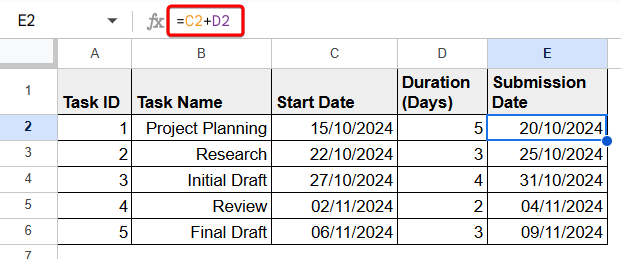
➤ Apply the following formula to add the task duration with the starting date:
=C2+D2
Thus, you will have the submission date automatically.
➤ To have the starting date of the next step of the project with a two days break, use the following formula:
=E2+2
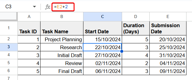
Similarly, you can plan the whole project automatically without inserting a single date manually.
Count Months Between Two Dates in Google Sheets
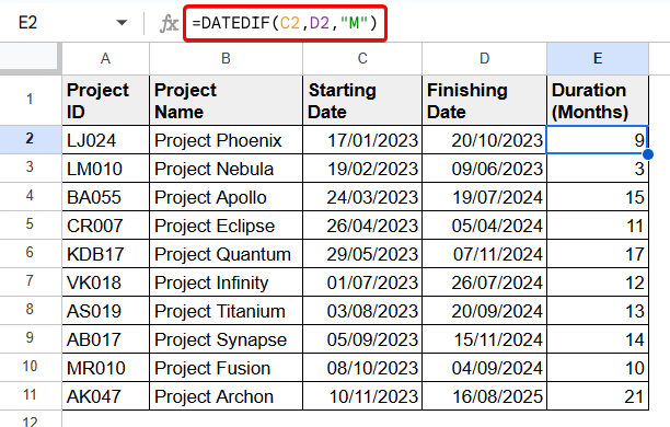
To count months between two dates in Google Sheets, you can use the DATEDIF function. While applying the DATEDIF function, you have to define the two dates and set the condition to find their difference in months.
Just use the following formula to count months between two dates:
=DATEDIF(C2,D2,"M")
Find Last Day of Month in Google Sheets
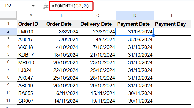
You can divide the process of finding the last day of a month in Google Sheets. You can use the EOMONTH function to find the last date of the month and the WEEKDAY function to convert the last date into day.
Follow the following steps to find the last day of the month easily:
➤ Use the following formula with the EOMONTH function to find the last date of the month:
=EOMONTH(C2,0)
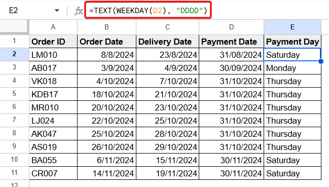
➤ Now, apply the following formula with the WEEKDAY and TEXT function to convert the last date of the month into day:
=TEXT(WEEKDAY(D2), "DDDD")
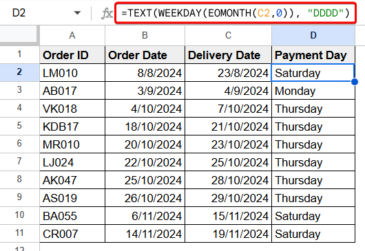
Alternatively, you can apply the following combined formula with the TEXT, WEEKDAY, and EOMONTH functions to find the last day of the month.
=TEXT(WEEKDAY(EOMONTH(C2,0)), "DDDD")
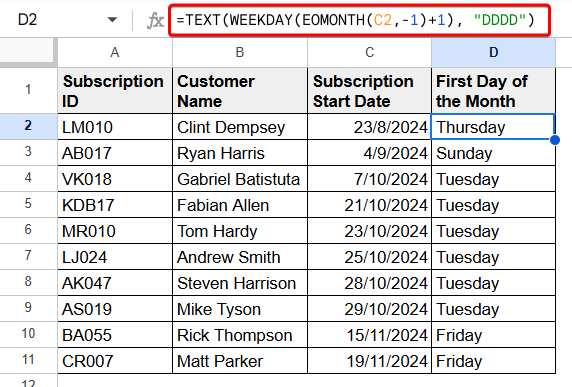
Find First Day of Month in Google Sheets
With a single combined formula with the TEXT, WEEKDAY, and EOMONTH functions, you can find the first day of a month at once.
Just apply the following formula to do so:
=TEXT(WEEKDAY(EOMONTH(C2,-1)+1), "DDDD")
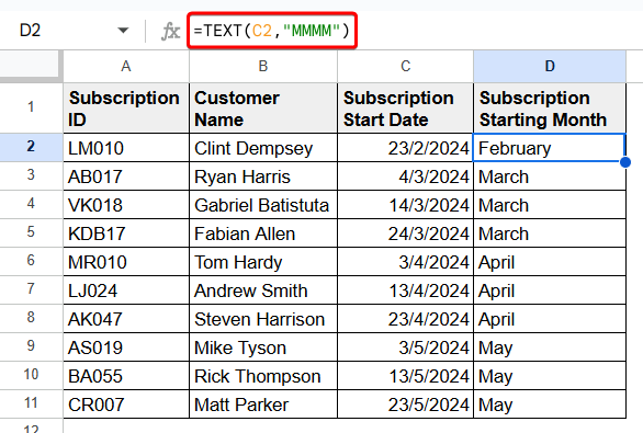
Find Month Name from a Date in Google Sheets
To find the month name from a date in Google Sheets, you can use the TEXT function. With just the TEXT function, you can easily do that.
Just apply the following formula to find the month name:
=TEXT(C2,"MMMM")
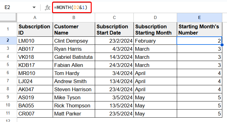
Convert Month Name to Number in Google Sheets
To convert a month name to number in Google Sheets, you just need to use the MONTH function and define the month name or the cell containing the month name.
Use the following formula to convert a month name to number:
=MONTH(D2&1)
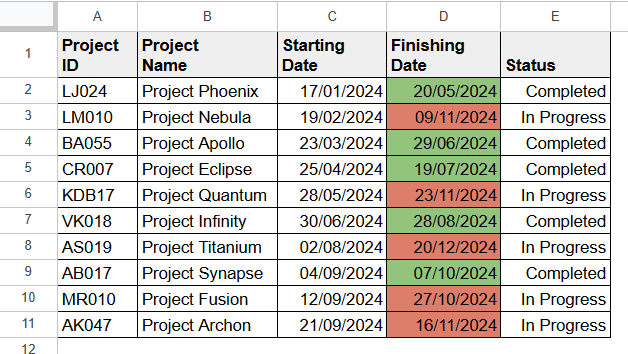
Applying Conditional Formatting on Dates in Google Sheets
Conditional Formatting enhances the visibility and readability of the dataset. You can apply conditions on dates to compare and format their cells easily on Google Sheets.
Follow the following procedures to apply conditional formatting based on dates:
➤ Select the dates first.
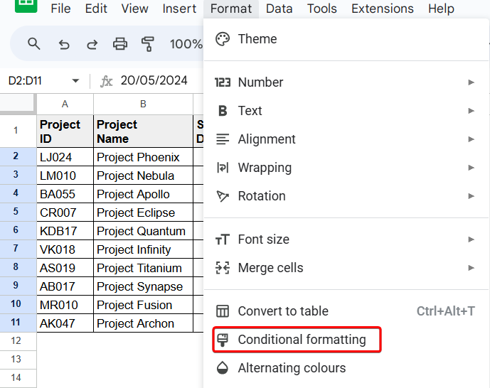
➤ Next, go to the Format.
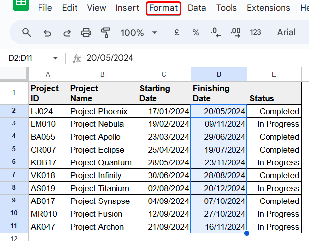
➤ Pick Conditional Formatting from the Format.
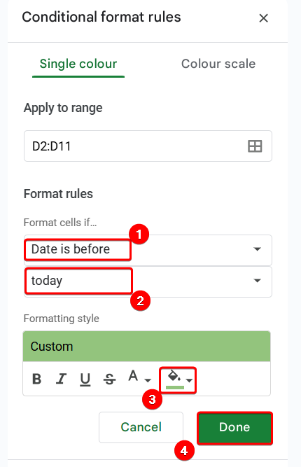
➤ From the Conditional format rules tab:
- Select Date is before first and then today from the Format cells if…
- Set a color for the matched values.
- Click on OK.
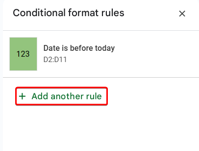
➤ To set another condition, click on Add another rule.
➤ Similarly, set Format rules and click on OK.
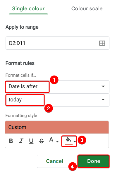
Thus, you can format your dataset applying conditional formatting based on dates.
Frequently Asked Questions
How to find the date from week number in Google Sheets where the week starts from sunday?
Based on the starting day of the week, the formula to find the date from week number in Google Sheets gets changed. You can use the following formula if you want find the date from week number where the week starts from sunday:
=DATE($C$1,1,1)+(A4-1)*7-(WEEKDAY(DATE($C$1,1,1)))+1
How to count days between two dates with DATEDIF in Google Sheets?
With the help of the DATEDIF function, you can count days between two dates in days. Use the following formula to have the days amount between two dates:
=DATEDIF(C2,D2,"D")
Concluding Words
The article discusses various Google Sheets date formulas used for manipulating and calculating dates. It explains different tasks like getting the current date, counting days between dates, and converting week numbers to actual dates. You can add or subtract days, find the first or last day of a month, and extract weekday or month names using specific formulas. The DATEDIF function helps calculate the difference between two dates, and EOMONTH is used to find the end of the month. It also describes how to apply conditional formatting to dates for better visibility and tracking. I hope this article is a great help for you.